Inventory management has been studied by many researchers and many practitioners. Tiacci and Saetta (2009) considered the relationship between forecasting and ordering policy with carrier capacity. Flores
Many researchers started studying the lost-sales model. In the case of stock-out, Gruen
Forecasting is never separate from inventory management. Liao and Chang (2010) investigated the effects of five demand forecasting methods, two inventory policies, and three lead times on the total inventory cost of a 3-echelon serial supply chain system. Tanaka
One expects that if a single ordering policy is applied to many different items with different shipping trends, the inventory would be a mix of items which has frequent shortages and those having excess inventory. On the other hand, even in using multiple ordering policies, it is not easy to find an appropriate policy for many types of items, particularly when each has a different shipping trend. In addition, given a particular shipping trend, no method or criteria has been specifically developed for choosing the ordering policy which would be applied to these items. For these reasons, the proper relationship between different item trends and the appropriate ordering policies is still not clear.
Therefore, we propose a new algorithm for finding a reasonable ordering policy using the relationships between shipping trends. In particular, our proposed algorithm classifies items according to shipping trends in order to find a suitable ordering policy and in addition reveals the shipping trends which are most desirable. In this case, shipping trends refer to shipping statistics related to the criteria of the ordering policy, which are calculated from past shipping data.
In section 2, we introduce the proposed model. The model development includes the converting of actual shipping data to data matrices for analysis. The details of the experiment and results of analysis are reported in section 3.
This study considers the inventory management problem for items having different shipping trends. Here, the ordering policyis assumed to perform differently according to item trends. To achieve efficient inventory management, we would like to select a suitable ordering policy for each item. Hence, we want to know which item trends are suitable for determining the ordering policy, or to find out a reasonable method for grouping which items would be suitable and which is not for a given ordering policy.
This study assumes that there has not yet been revealed a difference in item shipping trends and also what the suitable ordering policy should be. For deciding an ordering policy, the ideal case would be when the suitable ordering policy could be determined using only a single statistic. However, such a statistic is not yet known. Thus, many researchers have sought to find such a statistic based on theoretical considerations. Similarly, practitioners are also struggling to find such a trend.
In this study, we calculate and use shipping statistics and evaluation values of ordering policies. A general algorithm is presented in the following section.
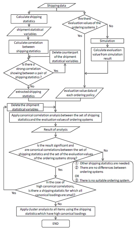
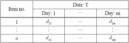
Figure 1 shows the flowchart of our proposed algorithm. First, we assume that there is shipping data, which informs shipping date and volume of items, like that shown in Table 1.

Shipping data
In the following steps, we repeatedly use multivariate data matrices, as shown in Table 2. Before we proceed to explaining the algorithm flowchart, we will first explain the premise behind multivariate data matrices.
Let X denote an
[Table 2.] General variable of each item
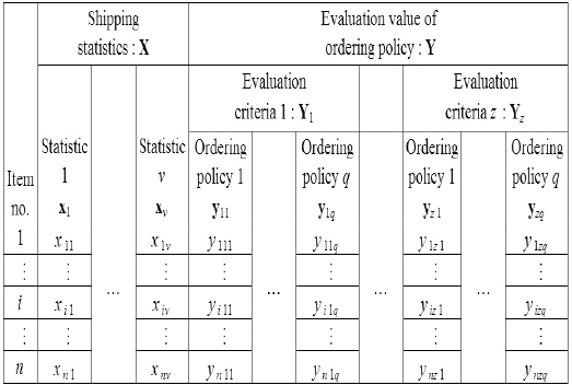
General variable of each item
Let Y denote the multivariate data matrix, which represents evaluation values of ordering policies. Y is similar to the previously mentioned X. For example,
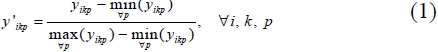
For analysis, since there are differences in the scale of numbers, we should standardize the evaluation value of each evaluation criteria and item in order to comparethe ordering policies. If
In order to evaluate multiple evaluation values, we apply a weighted linear mixed evaluate criteria. For example, if the criteria under evaluation are criterion
All the notations above, shown in Tables 1 and 2, are used in the sections that follow. The two large sets of variables, X and Y, are standard to, for example, the canonical correlation analysis and cluster analysis.
2.2.1 Canonical correlation analysis
The simplest known measure of relationships is the simple correlation coefficient between two variables. When interested in the relation between the set of variables X and a variable y, the multiple linear regression analysis can be used. However, in this study, we are interested in the correlation between the set of variables X and the set of variables Y, that is, each object for comparison has multiple variables. Canonical correlation analysis is one method for determining the relationship between sets of variables. According to Basu and Mandal( 2010), this was initially developed by Hotelling (1936).
The canonical correlation analysis focuses on the correlation between the
In the present study, we apply the canonical correlation analysis to the set of shipping statistics X and the evaluation values Y. In addition, we expect to find relationships between the sets of linear combinations of variables. This would allow us to sort shipping statistics into those which are significant and those which are not.
2.2.2 Cluster analysis
The cluster analysis is an exploratory technique. Cluster analysis techniques themselves can be broadly grouped into hierarchical clustering and non-hierarchical clustering. We here apply hierarchical clustering using the Ward method, which is a frequently used method.
In this study, we separate items into some number of clusters from xs, the shipping statistics, according to their relationship to Yi, the evaluation value of the criteria
Now, we calculate shipping statistics from actual shipping data and generate evaluation values of ordering policies from the simulation results. Then, we apply canonical correlation analysis to the set of shipping statistics and the evaluation values of the ordering policies. From these results, we can obtain the shipping statistics which exhibit a relatively strong relation with evaluation values of ordering policies. Clustering the items by these shipping statistics, we can group items according to a particular trend in the evaluation values of ordering policies.
In this study, we used SPSS ver. 19.0 (IBM Co., New York, NY, USA), a data mining and statistical analysis software package, for the canonical correlation analysis and cluster analysis, as well as the multiple linear regression analysis. The experimental environment is an Intel® Core™ 2 Duo CPU, E8400 at 3.00 GHz, 4.00 GB RAM; we did not need long computational times for our algorithm.
3.1 Ordering Policy and Experiment
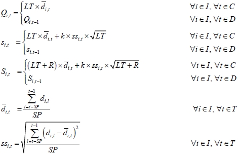
We used two ordering policies for this study: the so-called
For the
For the
In this study, we use

If practitioners would like to manage items precisely, it is necessary to shift ordering policy by some reason, like demand forecasting or seasonality. But, because we would like to find the relation between the shipping statistics values and the evaluation values of ordering policies, we did not shift ordering policies in the example applied.
In numerical and simulation experiments, we used the actual data of a distribution company’s shipments for the previous year. These items are categorized broadly into 11 varieties, for example, beer, Japanese sake, foods, and spices. In these categories, there are no obvious characteristic trends. So we selected about 5,000 items to be analyzed from about 7,000 items total. The other 2,000 items were less frequently shipped, and in smaller amounts. We applied our algorithm to the selected 5,000 items, those considered analyzable.
We simulated
We compared the performance between five ordering policies: the
From the results of the five ordering policy simulations, we define Y

We take the weights of shortage time,
Similarly, we define Yδ as the difference between evaluation values for criteria
between policy

We then apply canonical correlation analysis to the set of shipping statistics X and the set of evaluation criteria, using either Y
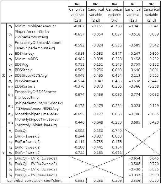
The results of the canonical correlation analysis are listed in Table 3. We apply the canonical analysis to the sets (σ, π ) and (σ, δ ), Here, σ is the set of shipping statistics and π is the set of evaluation values. The set δ is the set of differences in evaluation value. This notation is also used in Tables 4-6.

Canonical loadings (shipping statisticsevaluation value, differences between policy evaluation values)
Conducting the analysis shown in Table 3, we obtained the five canonical variables, ?π1, ? π 2, ?π3 , ? π 4 and ?π 5 from the canonical analysis of the sets (σ, π ) and four canonical variables, ?δ 1, ?δ 1, ?δ 2, ?δ 3 and ? δ4 from the canonical analysis of the sets (σ , δ ). We extracted as canonical variables only those for which the canonical correlation coefficient was at least 0.20, the value at which variables can be said to have a weak relation in terms of one group being affected by the other groups. Here, in addition to the canonical correlation coefficients, we must consider the absolute value of canonical loadings. If these are large in absolute value, then the statistic indicates a strong effect on the other groups. For example, in Table 3, if ?π 1 in X are listed in order of the strength of their relation to Y, then the canonical loadings are σ 6 = 0.751, σ 13 = -0.695 , σ 11 …. So, σ 6, which is the average of between the date of shipping (BDS), BDSAvg is the most significant statistic for the first canonical variable, ?π 1 of Y. And, if ? π 1 in Y are listed in order of their relation to X, these are π 5 = -0.732, = -0.558 , …. So, π 5, which is evaluation value (EV; R = 4 week, S), EV of
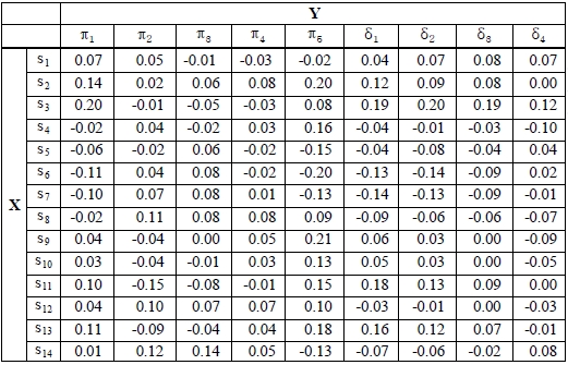
[Table 4.] Correlation between shipping statistics and evaluation value of ordering policy

Correlation between shipping statistics and evaluation value of ordering policy
The results of correlation analysis are listed in Table 4. In the Table 4, (σ6, π 2) represents the correlation of the average of BDS and EV of ordering policy
The last result is interesting in light of a comparison of Tables 3 and 4. Table 4 gives simple correlations of shipping statistics and evaluation values of ordering policies. By comparing these Tables, it is possible to say that no individual variables and evaluation values of an ordering policy clearly relate to each other. But individual groups of statistics and groups of evaluation values do. A comparison of Tables 3 and 5 reveals similar aspects, where Table 5 shows the results of the multiple linear regression analysis. For example, in Table 5, all entries of the σ13 and σ11 rows indicate a lack of a strong relation, whereas Table 3 does indicate a strong relation.

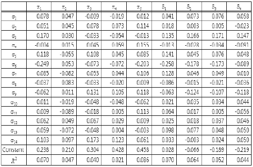
Standard partial regression coefficients of multiple linear regression analysis between the set of shipping statistics and each evaluation value
We, therefore, conjecture that searching for relationships between the set of shipping statistics and the ordering policies would produce results different than the other analyses.
By using cluster analysis, we separate all items into two groups, also called clusters. In Table 6, the averages of each statistic of each separated group, columns χα1 and χα2, and the averages of each statistic of all items, column χαall, are shown. In the cluster analysis, we use the Ward method and calculate distance of each itemfrom the statistics σ6, σ11, and σ13, those for which canonical correlation analysis results showed a relationship between shipping statistics and evaluation values of ordering policies in the canonical variable ?π1, the first canonical variable of canonical analysis to the sets (σ, π). The signs " + " and "?" to the right of the values for columns χα1 and χα2 are relative to χαall. For example, the value of (σ6, χα1) is higher than (σ6, χαall). Thus, the sign to the right, separated by a dashed, is " ." From Table 6, we can observe that there are trends within each cluster.
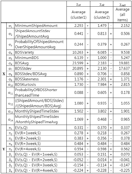
Statistical average of all items and two groups separated by the ward method (cluster analysis)
From the results shown in Table 3 and the σ rows in Table 6, it is possible to make predictions. For example, from looking at the ?π1 column of Table 3, let us consider σ6 , σ11 , and σ13 , which were the top three in terms of the strength of their relation in X to Y of column ?π1 In Table 3, the values of those σ’s , (σ6, ?π1), (σ11, ?π1), and (σ13, ?π1), are greater than zero, less than zero, and less than zero, respectively; thus, (σ6, ?π1), (σ11, ?π1), and (σ13, ?π1) correspond to ( , -, -). As another example, in the χα1 column of Table 6, the signs of (σ6, χα1 ), (σ11, χα1 ), and (σ13, χα1 ) are (+, -, -). Therefore, we can predict that (π1, χα1 ) and (π5, χα1 ) in Table 6 will follow the same tends as that represented in the ?π1 column of Table 3, that is, they will be less than the average.
In a similar way, in the ?π2 column of Table 3, let us consider σ8, σ12, and σ14, which were the top three in terms of the strength of their relation in X to Y of column ?π2 In Table 3, all three values were less than zero. In the χα2 column of Table 6, (σ8, χα2 ), (σ12, χα2 ), and (σ 14, χα2 ) correspond to (-, -, -). From these signs, we can predict that (π2, χα2 ) and (π3, χα2 ), and possibly (π4, χα2 ) and (π1, χα2 ) in Table 6, will follow the same trend as that represented in the ?π2 column of Table 3, which means they will be less than the average.
Next, in the ?π1 column of Table 3, (π6, ?π1 ), (π11, ?π1 ) and (π13, ?π1 ) have signs ( + , -, -); in the χα1 column of Table 6, (π6, χα1 ), (π11, χα1 ), and (π13, χα1 ) have the same signs, ( + , -, -). Thus, as we would predict, (π1, χα1 ), (π2, χα1 ), and (π3, χα1 ) in Table 6 would follow the same trend as that shown in the ?π1 column of Table 3, meaning they would be less than the average.
For the case of comparing the evaluation value of a policy, if the average performance of ordering policies were not significantly different and there are complementarities, such as π1 and π3, then a difference in evaluation values of ordering policies implies which ordering policy should be applied. For example, from Table 6, applying the original policy of the evaluation value π1, which is a
In this paper, our focus was on an approach to how to categorize items for a suitable ordering policy based on shipping statistics according to an evaluation of the ordering policy.
The practical point of view for real business of our proposed method is that practitioners can find, easily, significant shipping statistics values for selecting an ordering policy and can select an ordering policy for each item based on those significant statistics values efficiently. In the phase of finding significant shipping statistics values, we can look at the relation between the set of shipping statistics and the set of evaluation values of ordering policies.
In the numerical experiments, actual shipping data were used for calculating shipping data and simulating ordering policies. To evaluate the ordering policy, we considered the simulation results of
Using the results, we showed the effectiveness of grouping items by shipping statistics. Because groups, which are separated by cluster analysis, have different trends in evaluation values, it is possible to see how to select an ordering policy from shipping statistics. For example, by selecting ordering policies appropriately, we can reduce both shortage time and total daily stock.
Furthermore, we conjecture that the results of applying our method would vary according to the demand forecasting method, demand uncertainty, parameter settings for ordering policies, evaluation criteria settings and criteria of shifting ordering policy. By analyzing the interactions of these factors, we would like to extend the model beyond inventories to consider the global optimization of the performance of the entire supply chain management system.