As computer vision algorithms and computer aided lens design have continuously developed, the past twenty years have seen increasingly rapid advances in the field of aerial cameras which can calculate the distance or altitude [1-3]. Not only taking pictures but also measuring the distance of target objects has gradually been interested due to demand of the customer (VOC). The optical specification of an aerial lens is much tighter than any other applications such as mobile phone camera, vehicle camera. We consider the level of manufacturing difficulty and tolerance in order to optimize the optical performance in developing an aerial lens system. As shown below in Fig. 1, viewing angle is one of the important factors among optical specifications. It has a range from 20deg to 120deg. In this paper, we are focused on the lens system which has a 30deg viewing angle because there are some solutions to make wide angle such as image stitching and panoramic field of view algorithms.
When we consider an aerial camera which can calculate the distance or altitude through geographical features, the stereo camera is the most promising device in the field of topography analysis among other applications such as Lidar and Radar. However, compared with Lidar and Radar, the weak point of a stereo camera is detection range and distance accuracy. In this study, we focus on the way to improve optical performance enough to be adopted as an aerial camera. Finally, the aerial camera enables us to detect object distance within 10% error.
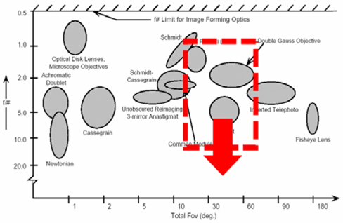
We can efficiently and easily choose an optical system by considering the functional dependence of an aberration for a change in f/number or field angle [4].
As shown below in Fig. 2, our target optical system will be triplet or double gauss in the viewpoint of FOV and f-number. At the initial step, we considered a triplet optical system in designing a lens system because triplet design is a more simple and efficient way than double gauss design.
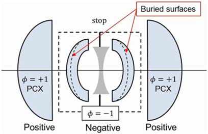
But MTF performance is not sufficient for the purpose of aerial topographic analysis. So, a double gauss lens which has two aspherical lens surfaces at the right and left sides of aperture(STOP) will be a good start point from the viewpoint of lens design because Mandler’s triplet model provides an effective way to realize the double gauss design. Generally, we use aspherical lens surfaces at both sides of the aperture in order to enhance MTF due to rule of thumb. Its process is simple and powerful in designing a variety of lens applications. Mandler’s triplet model was begun by the Cook triplet lens system. As shown below in Fig. 3, the second lens converts the negative element into meniscus type and split meniscus type into doublets for better optical performance.
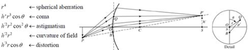
The optimization process will be carried out with the help of optical software Code-V. The main idea about optimization is the fact that the optical performance will be enhanced through minimization of ‘Seidel third aberration such as spherical aberration, coma, astigmatism, distortion. To maximize MTF performance, aberrations should be effectively removed. Imaging systems containing many aberrations lead to image degradation. These are aberrations that become prominent in third-order optics, also known as Seidel optics. The amount of aberration in a lens is related to semi-aperture r, the field angle Θ, and deviation from axial image h’ as follows in Fig. 4. [5].
Code-V has a merit function in order to optimize optical performance. It consists of many kinds of parameters such as RMS spot size, RMS wavefront, MTF and user defined. For example, the error function of MTF is Σ(weight^2)j x (MTFj – Targetj )^2 over the entire frequency. The value of the error function will be different depending on how many weight values set over each frequency. We don’t fully understand merit function due to the unknown weight values over the entire frequency determined by the internal algorithm of Code-V.
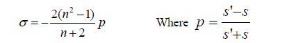
We can intuitively know improvement direction of optical performance by judging the positive or negative value of aberrations, whereas a conventional optimization method uses RMS errors which have no information on the direction of value. In order to minimize third-order Seidel aberrations, bending factor and the Coddington shape factor will be used to minimize the aberrations. The minimum spherical aberration can be realized if the bending factor becomes as below.

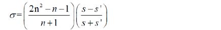
The coma aberration can be removed when the Coddington shape factor is the same as

In this study, we try to optimize refractive index and curvature of lens to minimize the aberrations.
Although the five monochromatic third-order Seidel aberrations provide us good insight regarding an optical system, tolerance parameters can enormously degrade the optical performance. Consequently, the aim of additional design including tolerance parameters is to verify that our design is less sensitive to many manufacturing deviations which degrade the image quality and to determine the acceptable variation which meets performance target. If the tolerances are considered as too narrow, other design may be required. The first step of tolerance analysis is to decide compensators and then set a standard of judgment such as MTF, RMS wave-front error and encircled energy. Compensators are the parameters which can be controlled in the assembly and alignment process. Conventional compensators are focus motion, axial motion of a lens or lens group, etc. Without compensators, the tolerances on the optics and mechanical parts will be unreasonably narrow. There are two kinds of tolerance. The one is manufacturing tolerance when a lensmaker produces a single optical element. It is composed of radii, surface figure (power, irregularity), special surface parameters (e.g., aspheric parameters), thickness (at vertex and of sag flats), index and dispersion and wedge. Another is assembling optical components into a system. It also includes axial displacements of an element or of a group, tilt and displacement of a single element, tilt and displacement of elements as a group. The next step of the tolerance process is a sensitivity analysis. It is the step of analyzing through sensitivity coefficients which consist of A and B. They are expressed as the function of MTF = A × T^2 + B × T + C. If the coefficients of A and B are larger than that of other factors, this factor is sensitive to tolerance variations. The parameters of A and B are used in order to analyze tolerance analysis [6-8].
The calculation of aberrations is impossible if there are a lot of lens elements because ‘third order Seidel aberrations’ have complex properties which consist of lens curvature, lens thickness, refractive index. To solve this problem, R.S.M is introduced with the purpose of obtaining much information with the minimum of experiments. According to Pareto’s law, the acceptable range of the vital few can be found through optimization by Response surface methods (R.S.M.). We can logically get the reasonable range of the vital few by using the Response Optimizer table of R.S.M. So, we can determine the reasonable range of the vital few which influence MTF.
Robust design will be useful in minimizing the performance variation of optical properties from the viewpoint of temperature. The selected noise levels should satisfy the range of conditions that the response variable should remain robust. We consider temperature variation as noise factor. Temperature change will cover the range from -30 degrees to 85 degrees. As temperature is changed, radius, thickness, refractive index of the lens system become prominently different compared with those of 25 degrees. We can easily simulate the variation by temperature change through thermal coefficients of expansion (dt/dT) and the rate of refractive index change (dn/dT) using an Excel program. For instance, TAF1 glass material has 4.85E-6 refractive index number and 6.6E-6 thermal coefficient of expansion. As temperature changes, we calculate the result as shown in Table 1 [9].
[Table 1.] Change of optical properties by the variation of temperature
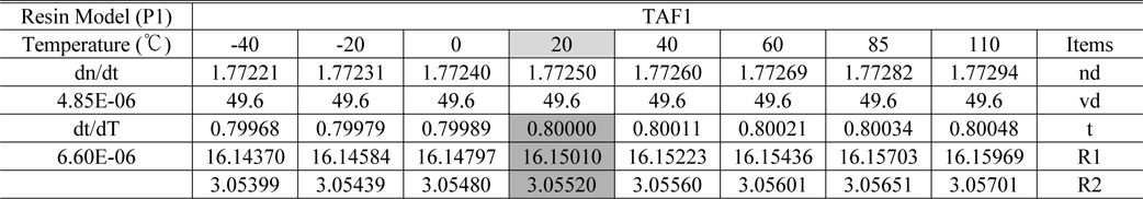
Change of optical properties by the variation of temperature
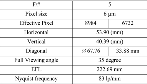
We make the specification for the proposed aerial lens, which has resolution of 60 mega pixels. This specification refers to conventional CMOS sensor data and viewing angle for aerial camera. The F-number of this system is 5.0 and overall length is 152 mm. Lens specification for aerial camera system has been set up as follows in Table 2.
[TABLE 2.] Lens specification for aerial camera system

Lens specification for aerial camera system
As mentioned earlier, we simulate lens design using double gauss configuration. Although double gauss configuration is well balanced in the viewpoint of aberrations as we predicted, the coma and spherical aberration are the greatly dominant factors in this system. So, we focus on eliminating the amount of coma and spherical aberration by using code-V macro.
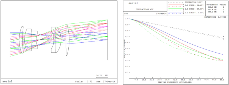
After minimizing the amount of spherical aberration and coma as below in Fig. 5 & Table 3, we can achieve MTF performance which is maintained more than 0.3 at Nyquist frequency, in comparison with initial lens design which is nearly zero regarding MTF as follows in Fig. 6 & Table 4. So, lens design using the third order Seidel aberration is effective and powerful when we optimize the lens system

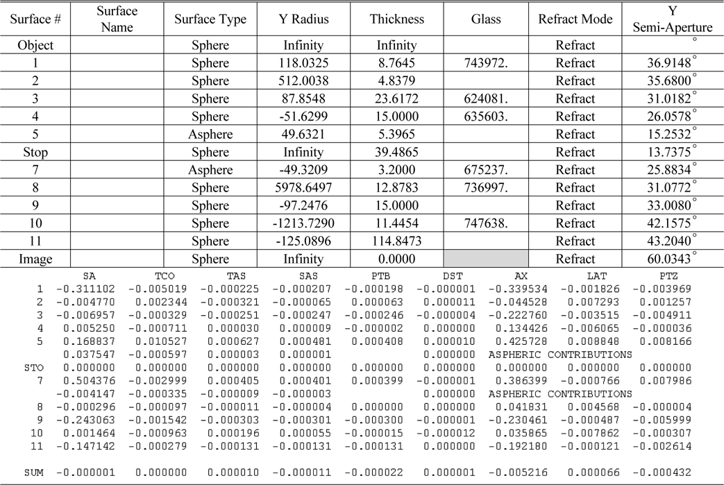
Third order aberrations of each lens surface after minimizing the amount of third order aberrations
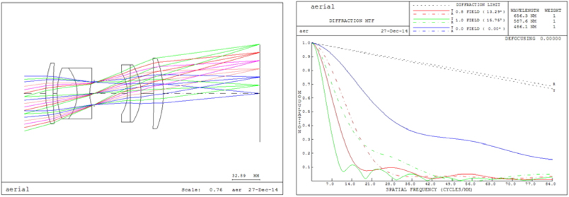
[TABLE 4.] Third order aberrations of each lens surface on the initial lens design stage
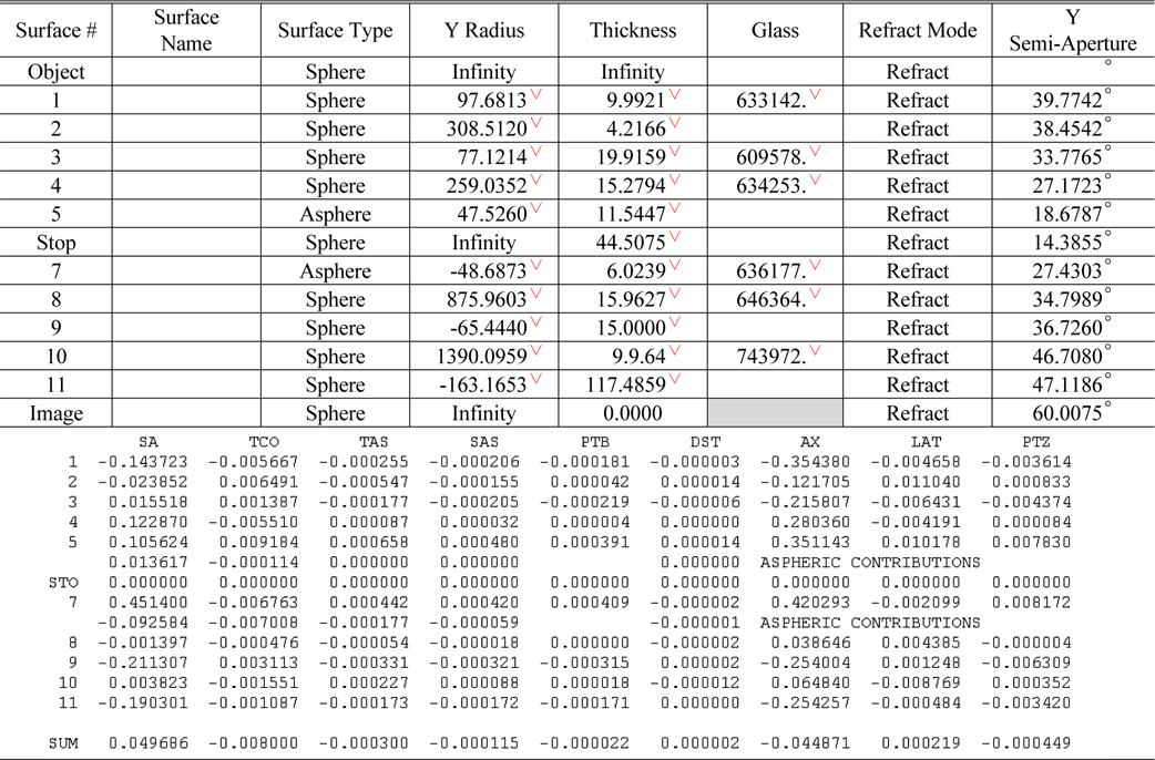
Third order aberrations of each lens surface on the initial lens design stage
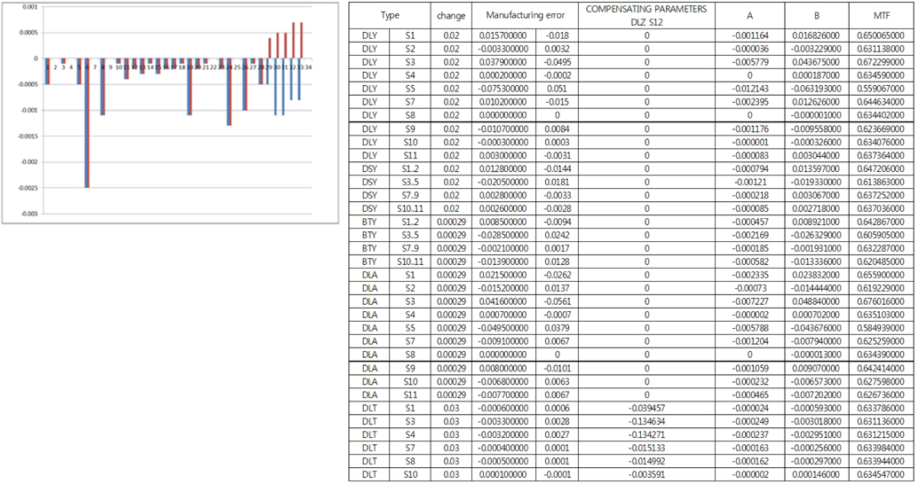
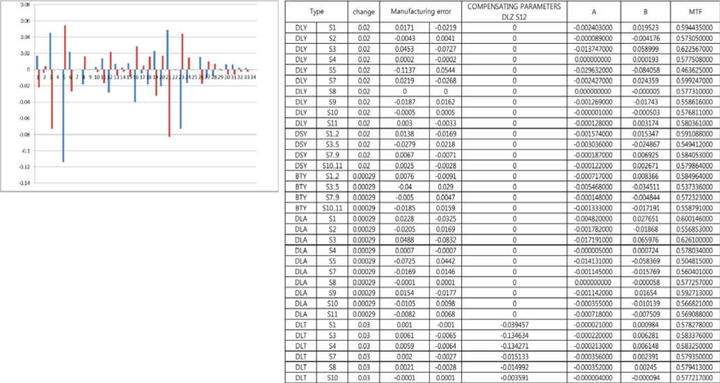
Sensitivity analysis is conducted for selecting vital few. For design flexibility, BFL (Back Focal Length) was adopted as compensator. Sensitivity coefficients are related to degrade MTF performance as the function of MTF = A × T^2 + B × T + C. The bigger the values of A and B, the more dramatically falls MTF. We analyze the sensitivity table of three fields (on axis, 0.5F & 0.8F) to optimize over the entire field following Figs. 7, 8 &9.
The fluctuation of MTF at the 0.8 field is much more sensitive than that of 0 field and 0.5 field as we thought. In conclusion, we can select ‘decenter and tilt of 2nd & 3rd lens’ as vital few. The factors will be DLY S3, DLY S4, DLY S5, DLA S3, DLA S4 & DLA S5.
As the next step, we are interested in selecting acceptable tolerance of DLY S3, DLY S4, DLY S5, DLA S3, DLA S4 and DLA S5, which stabilize the yield of mass production. We scrutinize optical performance at 0.8 field because the fluctuation of MTF at the 0.8 field is much more sensitive than that of 0 field and 0.5 field. Statistical analysis of simulation data using Minitab program is conducted through Response surface methodology as below in Table 5. Dependent variable is MTF and independent variables are DLY S3, DLY S4, DLY S5, DLA S3, DLA S4 & DLA S5.
[TABLE 5.] Experiment setting and results by R.S.M
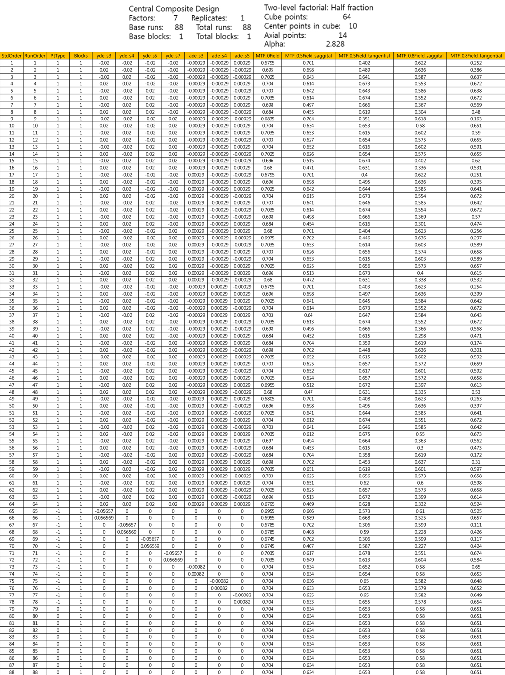
Experiment setting and results by R.S.M
Response surface methodology is used to analyze the relationship between one or more dependent variables and independent variables or factors. It is often conducted after vital few (controllable factors) is already known and it is usually chosen in suspecting curvature effect of MTF. We experimentally understand that optical elements such as lenses have the biggest non-linearity optical performance by variation of decenter, tilt & curvature. This is a new approach to conduct the tolerance analysis in the viewpoint of the statistical estimation scheme, even though Code-V can also do it. We can predict the effect of MTF by using two kinds of hypothesis such as null and alternative hypotheses. We can easily comprehend the effect of MTF for all combinations of every parameter through the analysis of response optimizer as below in Fig. 11. In other words, we can see the interaction effect through Response surface methodology.
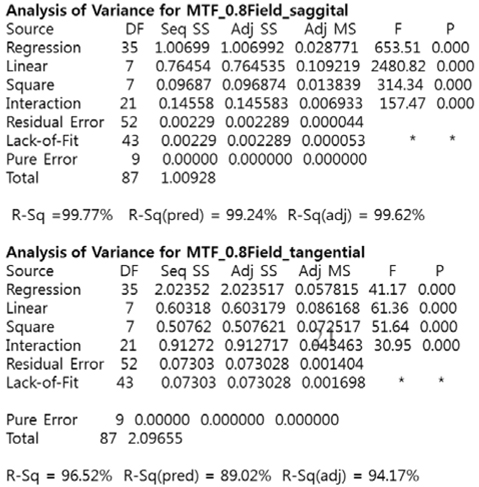
In the viewpoint of statistics as follows in Fig. 10, an alternative hypothesis that regression has significant meaning can be accepted due to the fact that the p-value of regression is 0.00. The explanation power of regression is 99.62% and 94.17% judging from R-sq(adj). We can reach a statistically reasonable conclusion from p-value and R-sq(adj). In addition, the pooling process which transfers unnecessary factors to pure error can be omitted due to the fact that all of the p-values are exactly zero [10].
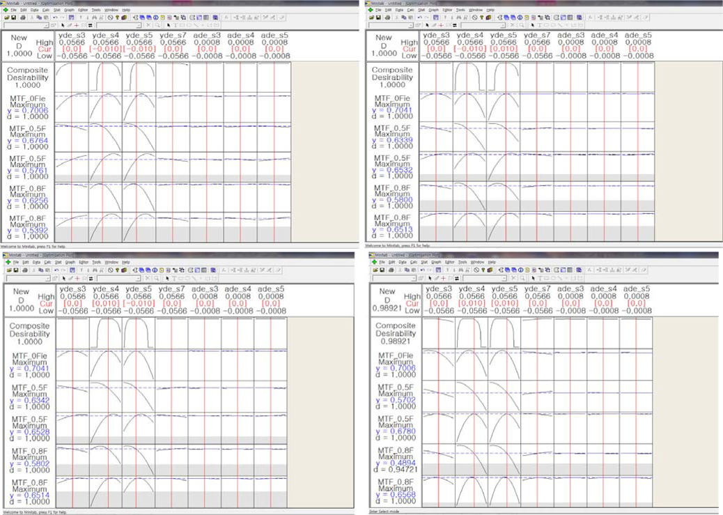
In the response optimizer graphs as follows in Fig. 11, decenter of S4 and S5 plays a vital role in maintaining MTF performance in this system.
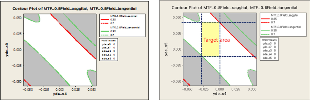
We can also detect the curvature effects at the decenter of S4 and S5 as follows in Fig. 12. Eventually, the manufacturing errors can be minimized by adjusting the variation of displacement of S4 and S5 within the reasonable range.
We can’t display all combinations of cases, so we will show the four cases including each ±0.01 decenter of 4th and 5th surface. In case 1, MTF will be 0.7 at on axis and 0.58 at 0.8 field on the condition that the decenter of −0.01 mm at the 4th surface and −0.01mm at the 5th surface. In case 2, MTF will be 0.7 at on axis and 0.61 at 0.8 field on the condition that the decenter of −0.01mm at the 4th surface and +0.01 mm at the 5th surface. In case 3, MTF will be 0.7 at on axis and 0.61 at 0.8 field on the condition that the decenter of +0.01 mm at the 4th surface and −0.01 mm at the 5th surface. In case 4, MTF will be 0.7 at on axis and 0.57 at 0.8 field on the condition that the decenter of +0.01 mm at the 4th surface and +0.01 mm at the 5th surface. To sum it up, we can obtain desirable lens design which is insensitive to tolerance variation by setting a limit on each ±0.01 decenter of 4th and 5th surface. All tolerances except the decenter of 4th and 5th surface should be maintained under standard tolerance.
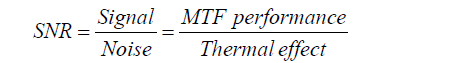
To obtain robust design which is insensitive to temperature variation, the Taguchi method is introduced [11]. It is possible for us to obtain quantitative measurement through SNR ratio. Higher values of the signal-to-noise ratio (S/N) identify control factor settings that minimize the effects of the noise factors.

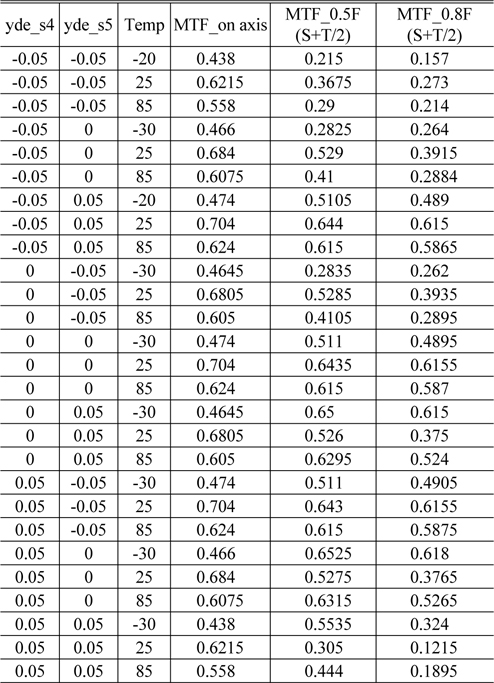
The decenter of S4 and S5 was selected as the vital few by RSM. We consider the decenter of S4 and S5 as control factors and temperature variation as noise factor. Temperature change will cover the range from −30 degrees to 85 degrees. We can easily simulate the variation of MTF by temperature change through thermal coefficients of expansion (dt/dT), the rate of refractive index change (dn/dT) using Excel program as follows in Table 2. This experiment is spontaneously provided through Minitab program as below in Table 6.
[TABLE 6.] Experiment setting and results by Taguchi method

Experiment setting and results by Taguchi method
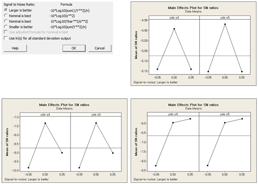
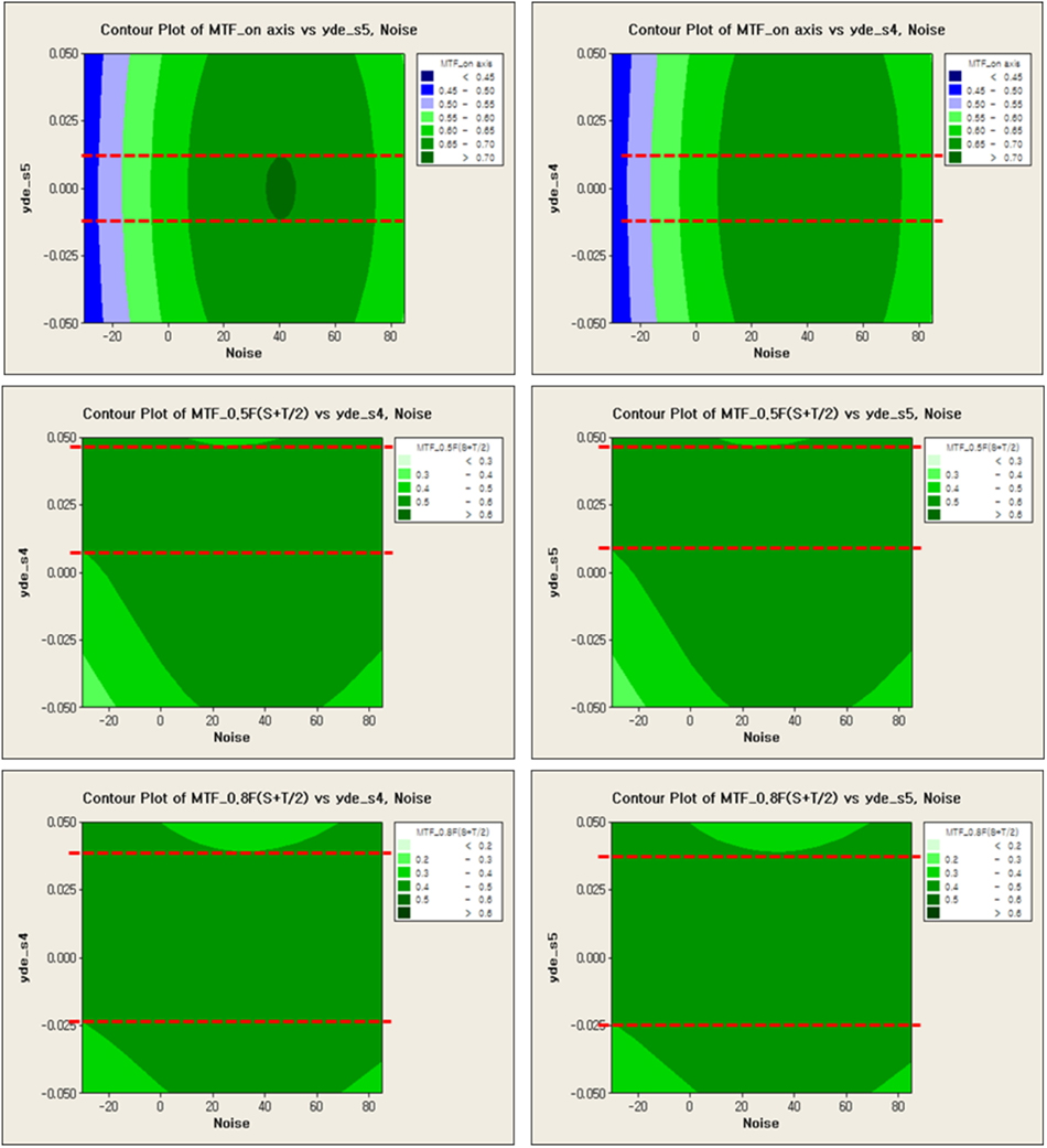
Optimal conditions can be selected by the signal-to-noise ratio which compares the level of a desired signal (vital few) to the level of background noise (temperature). From main effect plot and contour plot as follows in Fig. 13 & 14, we can reach the conclusion that the decenter of 4th and 5th surface should be controlled between 0 mm and 0.01 mm in order to guarantee robustness which is insensitive to temperature variation. This is a new approach to conduct the thermal analysis in the viewpoint of statistics, even though Code-V can also do it. We can conduct the quantitative analysis through the ratio of S.N.R (signal-to-noise). Taguchi designs are balanced, that is, no factor is weighted more or less in an experiment, thus allowing factors to be analyzed independently of each other. So, it allows us to analyze many factors with few runs.
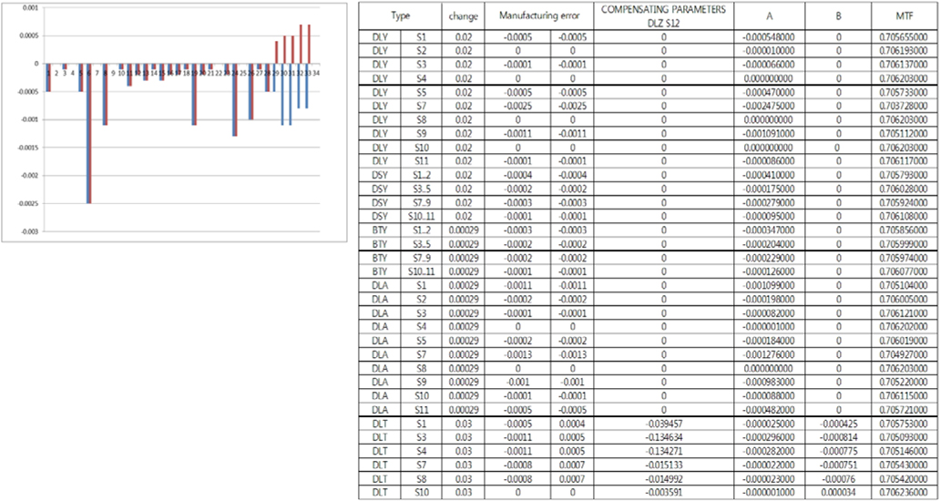
We will predict yield using cumulative probability to verify whether our proposed statistical analysis method works well or not. MTF analysis is conducted by tolerance factors as below in Table 7.
[TABLE 7.] The list of tolerance (left table: standard tolerance / right table: proposed tolerance)
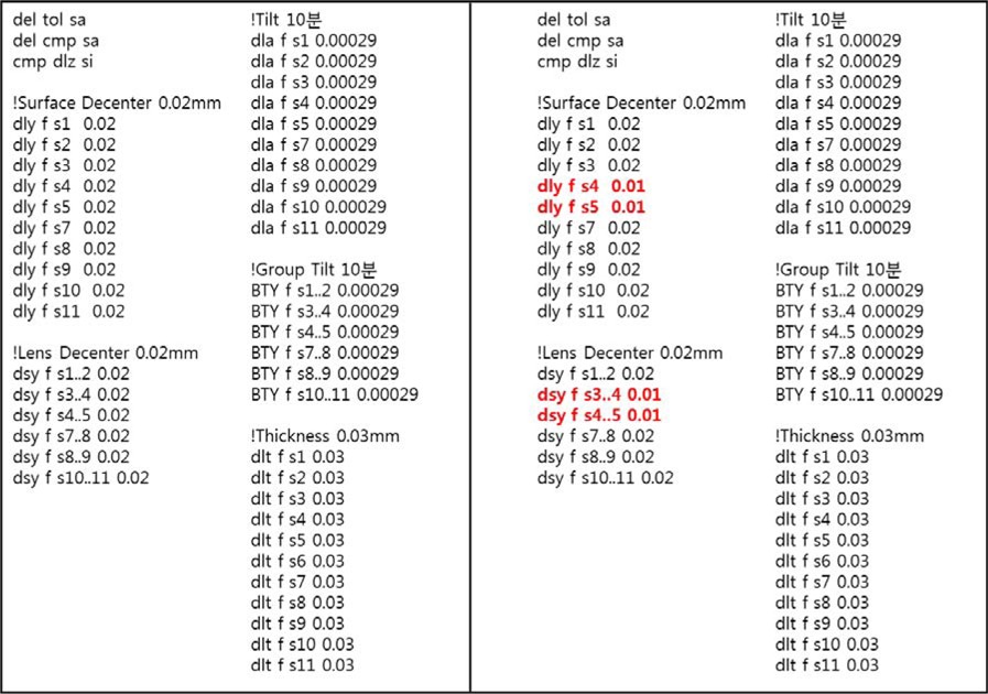
The list of tolerance (left table: standard tolerance / right table: proposed tolerance)
One is standard tolerance analysis. Another is proposed tolerance analysis considering the range of vital few that consists of decenter of 4th and 5th surface.
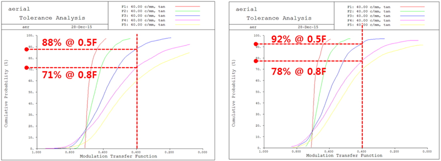
In the viewpoint of yield using cumulative probability as follows in Fig. 15, MTF performance of proposed tolerance is better than that of standard tolerance. Compared with standard cumulative probability of 71%, cumulative probability of 78% considering the range of vital few is remarkable improvement in that 43 tolerance factors such as decenter, tilt, thickness are applied.
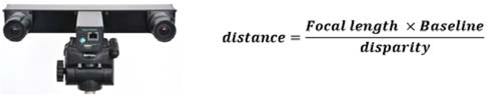
The formula for obtaining distance from two images can be briefly described as follows in Fig. 16.
Stereo camera system will get the information on distance as in the process below
1) Extract features from the left and right images
2) Match the left and right image features, to get their disparity in position
3) Use stereo disparity to compute distance
The image simulation of designed lens system is conducted by using the “2D image simulation function” supported by Code-V as follows in Fig. 17. In the skies of Yonsei University, the picture below was taken by aerial camera in 2014 (source: ‘http://aerogis.seoul.go.kr/app /mainfrm/ agis.do#’).
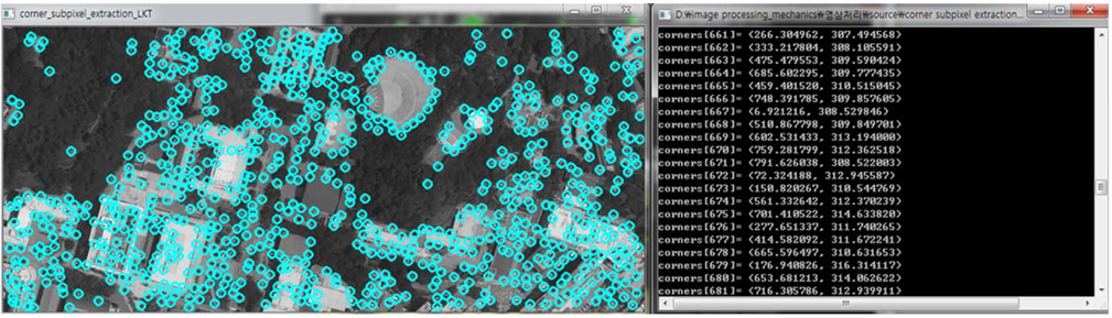
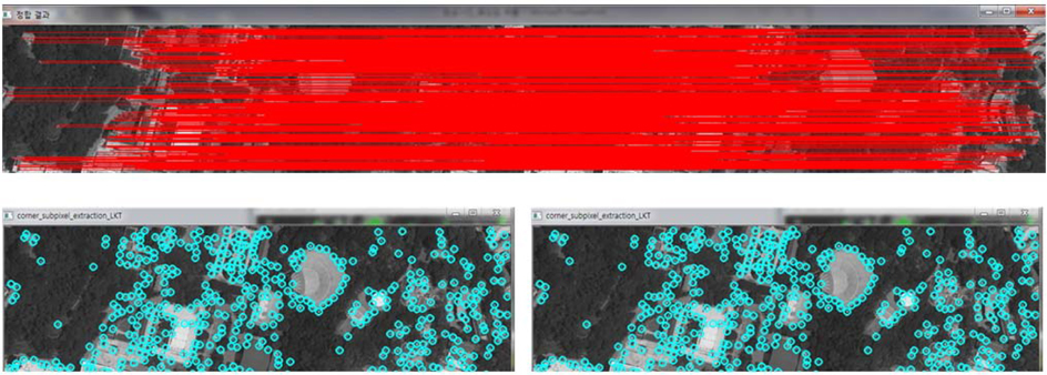
For extracting feature points, a sub-pixel extraction algorithm is implemented as below in Fig. 18. And then stereo matching algorithm is executed between left image and right image as shown in Fig. 19.
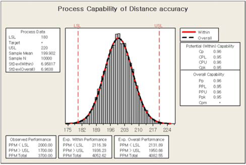
When proposed stereo camera system measures distance 200 m, the probability of distribution on the distance accuracy is displayed as shown in Fig. 20.
The 10000-trial Monte Carlo simulation was conducted to analyze distance accuracy performance within acceptable tolerance variation. The probability exceeding 10% distance error is 4092.55 ppm on the basis of long-term criteria
Finally, we come to the conclusion that proposed lens optimization effectively works well and successfully extracts geographical features in the aerial camera system.
The major objective of this study is to develop the lens system which is adequate for an aerial camera which can calculate altitude.
New concepts of lens design which reduce third order Seidel aberrations were suggested and simulated. In addition, statistical methodology is applied to optimize the optical performance such as RSM and Taguchi methods. This methodology is very efficient in that RSM can analyze the effect of MTF in case of all combinations and Taguchi method can obtain quantitative measurement through SNR ratio compared to the conventional way which is supported by code-V.
Finally, our design confirms that the result of the proposed lens design meets adequate specifications for the use of a dual aerial photograph.