Given the limits of the current policy framework, which include monetary and fiscal policies in the financial crises of the last decade, policy makers have searched for new macro policy to avoid crisisand mitigate large disruption in a crisis. Macroprudential policy is a strong candidate for the new macro policy. The new policy aims to control the behavior of banks such as lending and achieves stability in the entire financial system.
In practice, some international organizations have introduced macroprudential policy, such as the Basel III framework (Basel Committee on Banking Supervision (BCBS 2010, 2014). Under the Basel III framework, banks are required to satisfy a certain base level of capital ratio against risky assets to stabilize the volume of loan, and this base changes according to economic and financial conditions. Several countries have also introduced several types of macroprudential policies, including total credit control and capital control, as described in Lim
Some studies evaluate the roles of macroprudential policy using theoretical models including dynamic stochastic general equilibrium (DSGE) models. Schmitt-Grohe and Uribe (2012) develop a small open economy in which downward nominal wage rigidity pegging he nominal exchange rate induces a pecuniary externality. They show that under such an environment, the Ramsey optimal capital controls act as prudential policy in the sense that they tax capital inflows in good times and subsidize external borrowing in bad times. Eventually, this macroprudential policy reduces the average unemployment rate and average external debt, and increases welfare under reasonable parameters.
Quint and Rabanal (2011) assume a new Keynesian type DSGE model with real, nominal, and financial frictions; they study the optimal combination of monetary and macroprudential policies. They numerically show that the social welfare improves when the objective of the policy maker includes the credit term, which implies that the macroprudential policy is relevant. Suh (2012) shows that to improve welfare, macroprudential policy should respond to credit, whereas monetary policy should respond to the output gap and the inflation rate using the DSGE model with real, nominal, and financial frictions.
In this paper, we first develop a model with financial frictions by search and matching between firms and banks in the loan market as proposed by Fujimoto
The rest of the paper is organized into sections. We formulate the model in Section II. In Section III, we show the optimal criteria for policy. In Section IV, we show numerical examples of simple and optimal monetary/macroprudential policies for the Korean economy. Section V concludes the paper.
We exactly follow the model of Fujimoto
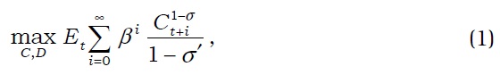
An infinitely lived representative household derives utility only from consumption, such that

where
In any period, a wholesale firm can either be a productive firm or a credit seeker firm. To be productive, a firm must first obtain credit
The credit market is characterized by search frictions, and a credit seeker firm must purchase retail goods
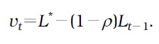
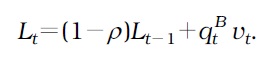
Banks post credit offers and search for credit seeker firms. We call these credit offers as “credit vacancies.” Posting credit vacancies is costless, but the total funds available for lending is fixed at

A credit vacancy is filled with probability . Then,

Credit market tightness is defined as
where
Retail firms produce differentiated retail goods from the wholesale good, which are then sold to the household. Wholesale firms are in a monopolistically competitive market. One unit of wholesale goods, whose price is , is converted into one unit of retail good
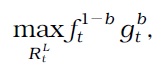
The number of new credit matches in a period is given by a Cobb-Douglas matching function
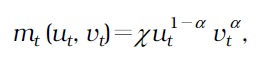
where

where
We log-linearize the structural equations around the efficient steadystate equilibrium as shown in the Appendix. For general stochastic nonefficient state, the Calvo-type stickiness introduced in the retail sector results into the standard Phillips curve with a cost-push shock ,
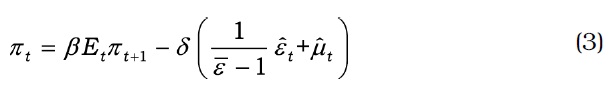
where
The retail price markup term in this equation can be obtained from the log-linearized version of Equation (29),

where
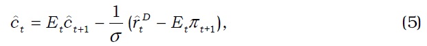
IS relation from equation (17) is given by

where we denote as the consumption gap.
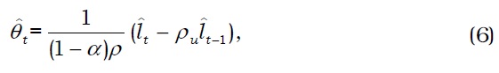
Using the loan volume term , the credit market tightness term is expressed as

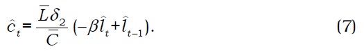
whereas the consumption gap is expressed as

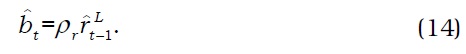
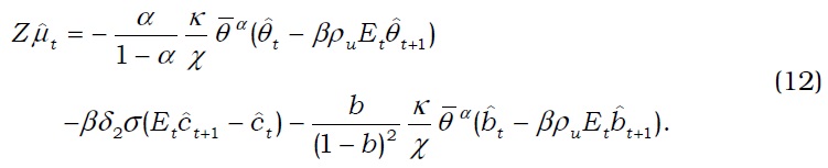
Although the closed linear system is given by the five equations and the monetary policy rule is derived in the subsequent sections, we can also reveal the relation between the loan interest rate and credit volume as
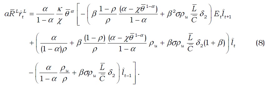
Thus, the loan interest rate and the volume of credit have a close relationship.
III. Optimality Criteria and Optimal Policy
Using linear-quadratic (LQ) approach of Woodford (2003) and Benigno and Woodford (2012), Fujimoto
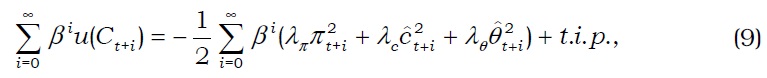
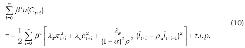
In detail, the second-order expansion of a household’s utility function around the efficient steady state is given by

where .
Fujimoto
Fujimoto

Thus, the optimal policy, including macroprudential policy, requires stabilization for volume of credit. When
1As the separation rate ρ approaches one, ρu approaches zero. 2As the separation rate ρ approaches zero, ρu approaches one.
Woodford (2003) shows that under the model with frictions in the goods market, that is, price stickiness, central banks should stabilize inflation and the consumption gaps, which roughly imply
By contrast, Fujimoto
In reality, some central banks pay attention to financial variables to implement the monetary policy under situations in which frictions in the financial market matter. For example, Taylor (2008) points out that a spread-adjusted Taylor rule that also includes the credit spread term in the standard Taylor rule can explain the easing of monetary policy by FRB in response to subprime mortgage crisis.
Therefore, we investigate whether adjusted Taylor rules achieve higher welfare than the Taylor rule does in the model with credit market frictions.
V. Implementation of Optimal Policy for Financial Stability
>
A. Calibration for Korean Economy
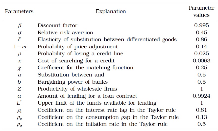
The model period is one quarter. We use the structural parameters in Table 1 for the Korean economy. Following Choi and Hur (2014), we set the relative risk aversion

PARAMETER VALUES
For other parameters, we assume
We set
In simulation, we assume a positive 1% cost-push shock in the Phillips curve with persistence of 0.5.
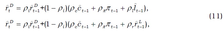
We check the performance of a variety of simple rules, namely, an estimated Taylor rule (TR), an estimated Taylor rule with a credit volume term (TRC), and an estimated Taylor rule with a loan interest rate term (TRL). TRC and TRL are given by

where
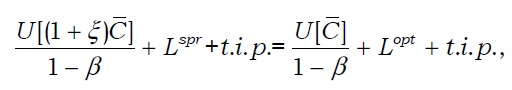
In numerical simulations, we search for

where
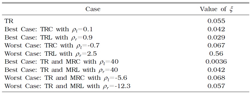
WELFARE ANALYSIS
The findings in the simulations are as follows. First, TRC and TRL perform better than TR under appropriate choices of parameters. In our exercise, TRC (TRL) shows the best performance, with
Inflation variability, consumption variability, and credit variables in the best TRC and TRL reported above have relative importance. The values of
We also check the performance of the simple macroprudential policy rule combined with TR. Here, we assume that the macroprudential authority aims to stabilize only the loan volume, such that the credit variation is the unique explanatory variable. This situation follows the conventional view of macroprudential policy. For example, the new Basel regulation imposes capital requirement on banks to primarily control the loan volume as in BCBS (2010, 2014). Moreover, Drehmann, Borio, and Tsatsaronis (2012) show that the variation of credit can be a good indicator to implement a macroprudential policy. We also consider the case in which the credit variation is replaced by the loan interest rate. More precisely, we assume that the macroprudential authority controls the bank’s bargaining power
The simple macroprudential policy rules are given by

We call these simple macroprudential rules as the macroprudential rule with credit variation (MRC) and the macroprudential rule with loan rate variation (MRL). By contrast, the central bank is only responsible for the stability of inflation and the consumption gap. Thus, we assume TR for the monetary policy.
The range of the policy parameters examined is -40≤
However, under inappropriate parameters, MRC (MRL) performs worse than TR, with
>
C. Change for Average Duration of a Credit Match
For sensitivity analysis, we change the average duration of a credit match to five years. Thus, we set
[TABLE 3] WELFARE ANALYSIS: SENSITIVITY FOR ρ

WELFARE ANALYSIS: SENSITIVITY FOR ρ
First, welfare improves and deteriorates with TRC, TRL, MRC, and MRL in some cases. Thus, parameter settings are important to achieve welfare improvements. Second, TRL shows better performance than TRC. Third, MRC performs better than MRL. These results have some robustness.
>
D. Change in Range of Search for Optimal Parameters
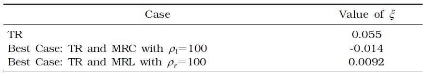
We now expand the range of search for optimal parameters because the optimal parameters for MRC and MRL are at the upper bound of the range. The range of the policy parameters examined has expanded to -100≤
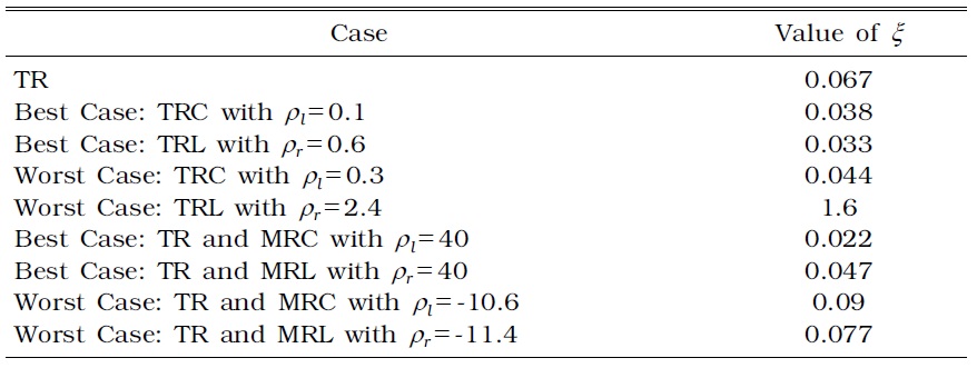
[TABLE 4] WELFARE ANALYSIS: SENSITIVITY FOR THE RANGE OF SEARCH FOR PARAMETERS

WELFARE ANALYSIS: SENSITIVITY FOR THE RANGE OF SEARCH FOR PARAMETERS
Interestingly, MRC with
3In this case, a is 0.9918 and κ is 0.0059 with other parameters unchanged.
We show that the simple macroprudential and monetary policy rules with credit terms can induce higher welfare than the estimated Taylor rule under the parameters calibrated for the Korean economy. Thus, an introduction of simple macroprudential policy in addition to the monetary policy can improve welfare in the Korean economy.
The following points could be of interest for future research. By extending the model into an open economy, utilizing optimal capital control as the optimal macroprudential policy becomes possible. In this case, it would be interesting to investigate the dynamics of exchange rate under capital control.