Over the years, several proposals of what it means to implement a computation have been advanced by philosophers (e.g., see Stabler 1987; Dietrich 1990; Chalmers 1994, 1996; Copeland 1996; Scheutz 1999, 2001). Since definitions of implemention are often cast in more general terms so as to not be forced to make commitments to particular notions of computation (or the notion of computation at all, for that matter), it is common to read about the “function(s) being implemented/realized by a physical system” instead of “the computation(s) implemented by a physical system.” Stabler (1987) presents, what could be called the “standard account of what it is to realize a function”:

Formally, this can be written as follows:

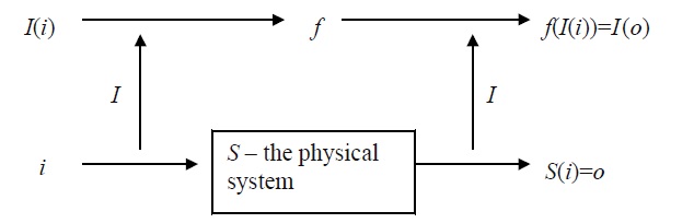
Definition 1: Let S be a physical system and f a function. S computes f if, and only if,

While this definition is very general in that it includes various other accounts of implementation and physical realization as special cases, the standard account of implementation, as it stands, does not quite work unfortunately. It has been pointed out that it is “too liberal,” for it does not put any restriction on the interpretation function: without any restrictions and constraints, every system can be viewed as implementing every computation (e.g., see the well-known arguments advanced by Putnam 1988 and Searle 1990 to that effect). Finding constraints that prevent the standard account of implementation from being vacuous is crucial to computationalism, the view that mental processes can be seen to be computational processes, as otherwise – if everything can be viewed as computing every function – computationalism loses its explanatory force (e.g., Chalmers 1994; Scheutz 1999).

One prima facie difficulty of the standard account is that “terms like ‘state’ and even ‘physical state’ tend to be used very loosely in this sort of context” (Stabler 1987, p. 3). Stabler demonstrates potential problems with the standard account by defining a special kind of physical state: assume the behavior F of a given physical system S can be described in a physical theory P (as long as certain background conditions C obtain that make this description applicable). Suppose further that an infinite sequence of timest₁, t₂, t₃, … is given. Infinitely many “physical states” can then be specified by stipulating that the system is in state p_i if and only if it satisfies its description F at time t_i. If the p_i are then taken to be the computationally relevant states, the system will “compute” any function f over the natural number. Define the interpretation I (for an arbitrary function f over the natural numbers) to be

Then S computes f by going through a sequence of states that are states by virtue of its description F being true of S at the respective time (under conditions C). In a sense, S does not really “compute f” but rather “enumerates” the pairs <i, f(i)> at any two successive points in time:

To see what needs to be done in order to “exclude tricks of this sort,” one needs to analyze different kinds of “tricks” and hope to be able to detect “common patterns.” It is clear that there must be “some restrictions on the interpretation function used in any empirically substantial computational claim” (Stabler, p. 4). Intuitively, one obvious problem with the above definition seems to be that states are picked out by particular times to obtain infinitely many computational states that could correspond to the infinitely many pairs of natural numbers that define f. But what if the computationally relevant states have to be “somehow extracted” from a physical description of the system?

Besides the question, whether physical systems can realize infinite functions at all (e.g., using infinitely many states), it seems that one has to account at least for cases like the calculator and revise the standard account to allow it to realize an infinite function using finitely many states. The idea is that infinitely many computational states are not needed to realize an infinite function if each argument of the function corresponds to a finite sequence of computational states. In other words, each natural number (that is an argument of f) would be “represented” by an input sequence of a finite number of computational states, and by the same token, each value of f for a given argument would correspond to an output sequence of finitely many states. The revised standard account, which allows a system with only finitely many (computationally relevant) states to realize an infinite function is presented by Stabler as follows:

Definition 2: [Revised standard account] Let S be a physical system and f a function. S computes f if, and only if,

Note that the revised standard account has made two crucial transitions: an explicit transition from (potentially) infinite sets of physical states to finite such sets, and another tacit transition from “physical states of the system” to sets of “physical input states of the system” and “physical output states of the system.” This is especially noteworthy as the latter account implicitly excludes so-called “inner states” of the system (which the former implicitly included): only the input-output mapping matters in the revised standard account as succinctly expressed by the formula Out (seq_o) = f(In(seq_i)). Put differently, the physical system is considered a black box, whose “inner mechanisms/workings” (as described by a physical theory) are abstracted over. Thus, while the revised standard account can answer the “what” question (i.e., “what function does a physical system realize”), it will not be able to answer the “how” question (i.e., “how does a physical system realize the function”), because it only takes input and output states from the physical theory (in which the system is described) ignoring the rest – hence, to account for the “how” question as well, more of the physical description of the system (than merely sets of input and output states) needs to be retained in the definition of “physical realization of a function.”

There are other modifications to Definition 2 that become necessary upon further analysis. For example, it has been pointed out by Kripke (1981) that a physical machine can only “approximately” or “imperfectly” realize an infinite function, for one, because time is limited (“it will run out of time”) and also because it will make errors (“nothing is perfect”):

Kripke’s objection to the general idea of a physical system realizing an infinite function rests on the claim that “indefinitely many programs extend the actual behavior of the machine” and that reference to intention of the designer (of a computing device) is needed to fix one particular program. To counter objections of that sort, Stabler suggests modifying part 2 of Definition 2 by adding the counterfactual clause “if the system satisfied conditions of normal operation N for long enough”:

By adding this clause, reference to the designer’s intentions is replaced by onditions of normal operation, thus avoiding the problems that the former aises for the functionalist (see Stabler, 1987, p. 19). Stabler, being aware hat introducing counterfactuals can cause more (additional) problems than hey can solve (e.g., see Putnam’s discussion of Lewis’ notion of causation n his 1988), argues that the kinds of counterfactuals involved in the conditions of normal operation are supported by physical laws:

Although it would be preferable to dispense with counterfactuals in an account of physical realization altogether (e.g., see Scheutz 1999), it seems that counterfactuals will always enter the picture if a notion of “normal operation” is involved (e.g., “if the system had been in condition C at time t, then…”). And such a notion of normal operation seems to take care of problems regarding potential malfunctions of a system (i.e., malfunctions with respect to the program that was supposed to describe the systems behavior, as noted by Kripke). Moreover, Stabler uses counterfactuals also to address Kripke’s first objection, namely that finite systems cannot realize infinite functions. His strategy to determine which infinite function a system realizes is to “couterfactually extend the life-time of a physical system”: if the system satisfied conditions of normal operation N for long enough, then it would be able to compute all pairs of a (particular) infinite function f.

Thus, with the modified standard account of implementation (2 + 2’), we are now in a position to analyze Chalmers’ notion of implementation.

Chalmers’ (1994) basic conception of how a computation is connected to the physical is an instance of the standard account of implementation where computations are set in correspondence with reliable causal transitions between physical states—f(→)=“reliably causes” (where ‘→’ is the formal state transition relation in the “computation,” an automaton, for example). To be precise, Chalmers actually provides two definitions of implementation, an informal and a (more) formal one, which he holds equivalent. It is worthwhile examining both, since they are not only cast differently, but also differ semantically. The first informal definition (which itself consists of two phrasings) reads as follows:

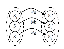
There is a little ambiguity in the two phrasings as to what the exact meaning of “mirrors” is supposed to be. Prima facie one would expect “mirrors” to mean something like “is isomorphic to,” as “mirrors” usually indicates sameness in structure:

Definition 3: [Isomorphism two algebraic structures with one relation] Let M₁=<D₁, R₁> and M₂=<D₂, R₂> be two structures with domains D₁ and D₂, respectively, where relation R₁ is defined over D₁×D₁ and relation R₂ is defined over D₂×D₂. These structures are then said to be isomorphic if there exists a bijective function f from D₁ to D₂ such that for all x, y∈D₁:

Yet, the second phrasing does not seem to imply structural sameness, since it requires only [iso⇒] (i.e., that “formal states related by an abstract statetransition relation are mapped onto physical states-types related by a corresponding causal state-transition relation”), but not the other direction [iso⇐] (i.e., that physical states-types related by the corresponding causal state-transition relation have to be mapped onto formal states related by an abstract state-transition relation, too). Hence, with “mirrors” Chalmers seems to mean only [iso⇒]. At a different place in the text, however, he suggests [iso⇐] when he writes “… that the formal state-transitional structure of the computation mirrors the causal state-transitional structure of the physical system” (1994, p. 393). So, it seems that “mirrors” is to be understood as “isomorphic to,” and, indeed, he later writes: “the relation between an implemented computation and an implementing system is one of isomorphism between the formal structure of the former and the causal structure of the latter” (1994, p. 396).

Hence, the mapping between physical state types and computational states has to be bijective (one-to-one and onto) and preserve the abstract state transition relation as well as the causal state transition relation in order to give rise to an isomorphism between computational and physical state types. Note that the existence of a grouping of physical states of the system into state types is required as a necessary prerequisite for the mapping to work and that there are no restrictions imposed on the grouping; its mere existence is sufficient.

Before we discuss Chalmers’ second (formal) definition, a remark on the use of the term “state” seems appropriate. The term “state” in this context is sometimes used in the sense of “token of a particular state type,” although this is at best ambiguous and misleading. “Automaton state,” for example, could denote a state in the set of states in the definition of the automaton as well as a state in a particular run of the automaton—the former is a type, the latter a token. 1 In physical systems, “physical state” refers to the particular physical makeup of a system at a time (under certain environmental conditions): if the system is described in terms of a system of differential equations O_m(t)=F_m(I₁(t), …, I_n(t), P₁(t), …, P_k(t)) (for finitely many m), then by fixing the time parameter (e.g., at t₁₇) one obtains the state of the system (i.e., by fixing the environmental conditions I₁(t₁₇), …, I_n(t₁₇), one obtains P₁(t₁₇), …, P_k(t₁₇) as well as F_m(I₁(t₁₇), …, I_n(t₁₇), P₁(t₁₇), …, P_k(t₁₇)) for all m). For example, physical states in field theory would correspond to the value of all field parameters at a given time. This notion of state is independent of how often it is instantiated by the system (if at all).

Yet, some philosophers still use “state” as if it referred to a unique particular physical occurrence, a constellation of a physical system which obtains only once at a particular moment in time, and thus once in the life-time of the system. 2 While nothing can be identical to this particular occurrence (and it, therefore, does not make sense to say things like “this occurrence is the same as x”), the above usage of “state” supports a notion of “sameness” (e.g., the system was in the same state at time t₁₇ and t₁₇). Thus, a physical state is not a (concrete) token of some physical state type, but rather a type itself.

To avoid terminological (and consequently conceptual) confusion, we will use the term “instantiation of a state” (or maybe “state token,” e.g., see Melnyk, 1996) to refer to a unique physical occurrence, and the term “state” in all other cases. The term “physical state type” will be used to stress that a particular physical state has been obtained by type formation from “simpler states (state types).”

After having explicated the overall structure of “implementation” in the first definition, Chalmers spells out the details in a more formal definition in which he uses a finite state automaton (FSA) as a representative for other computational formalisms:

Note that nothing in this definition requires that the mapping f be one-toone, the reason being that imposing injectivity on f does not seem justifiable in the light of multiple realization arguments. Just consider an ORgate, where the potential, which is supposed to correspond to “1,” fluctuates between 4.5 and 5.5 Volts (where 5 Volts would be the “ideal” voltage). In this case, there is a whole set of physical states, which are all different from each other, yet “similar enough” to be rightfully taken to correspond to “1,” as practice shows. Hardware designers do it all the time; they produce functioning machines whose computational description works both as explanation and prediction of the machine’s behavior. Yet, such a correspondence between one computational state and many physical states would be excluded by the restriction that f be one-to-one.

This is where the idea of a grouping of physical states (mentioned in the former definition) comes to reconcile two seemingly incompatible ideas: 1) that no one-to-one correspondence can be established at the level of physical states (for the above and similar reasons), and 2) that the computational description is supposed to mirror the causal structure of the physical system. By relating not the physical states themselves, but more complex types of these states (formed by the “particular grouping” of states into types), it becomes possible to establish a one-to-one and onto relationship between these types and computational states, which is the prerequisite of an “isomorphism” (the mathematical term expressing structural identity, i.e., “mirroring”).

Chalmers, although never explicitly, seems to suggest that it is possible to obtain a bijective mapping f* from f that will give rise to an isomorphism between the physical system and the formal computation by collecting all those states s to form a state type [s_i] that are mapped onto the same automaton state type S_i according to f: “The state-types can be recovered, however: each [s_i] corresponds to a set {s | f(s)=S_i} for each S_i∈M. From here we see that the definitions are equivalent. The causal relations between physical state-types will precisely mirror the abstract relations between formal states.” (Chalmers, 1994, p. 393) One would define f* from physical state types onto computational state types such that f*([s_i])=S_i for each S_i∈M. This mapping is one-to-one because the physical state types have just been defined as such, and it is, furthermore, onto (ensured by the “for every state transition relation”-clause in the definition), but it is not isomorphic, since even though [iso⇐] holds (because of the “conditional”), [iso⇒] does not necessarily hold. I.e., there can be reliable state transitions from all physical states [s_i] upon input i into states [s’_i] producing output o’ for which corresponding states f*([s_i])=S_i, f*([s’_i])=S’_i, f(i)=I, f(o’)=O’ exist without there being a state transition (S, I)→(S,’ O’) in M.

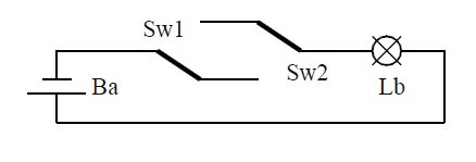
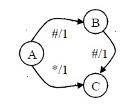
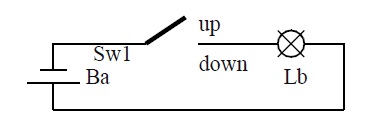
To see why Chalmers’ definition fails to capture his view about “mirroring” (i.e., isomorphism between physical and formal structures), let us examine how his definition works in detail, starting with a simple physical system P₁ (e.g., described in circuit theory—see Figure 2) for which we can easily specify physical states types: switch Sw1 is connected to light bulb Lb and battery Ba by copper wires.

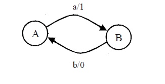
Input to P₁ consists in switching Sw1 from either “up” to “down” or vice versa (the states are named ‘1u’ for “Sw1 upwards,” ‘1d’ for “Sw1 downwards”). The internal states of P₁ are the states of Sw1 (‘u’ for “up,” ‘d’ for “down”). Finally, output produced by P₁ are the states of the Lb which is either lit or or not lit (‘+’ for “light on,” “-” for “light off”). Now consider the following automaton M₁=<Q, Σ, Γ, δ, q₀, F>, where Q={A, B} is the set of inner states, Σ={a, b} the input alphabet, Γ={0, 1} the output alphabet, δ={<, >, <, >} the transition function from states and inputs to states and outputs, q₀=A the start state, and F={A, B} the set of final states (which in this case does not really matter). The automaton is depicted (in the standard fashion) as a graph in Figure 3, where nodes denote states and edges denote transitions between states, both labeled accordingly (the format for edge labels is “input/output”). For the rest of the paper, we will represent automata using graphs instead of the more tedious mathematical notations.

Automaton M₁ transits from state ‘A’ on input ‘a’ to state ‘B’ outputting ‘1,’ and from state B on input ‘b’ to state ‘A’ with output ‘0.’ It follows that P₁ implements M₁ according to Chalmers’ definition; just map (every occurrence of) “u” to ‘A,’ (every occurrence of) “d” to ‘B,’ (every occurrence of) “1d” to ‘a,’ (every occurrence of) “1u” to ‘b,’ (every occurrence of) “+” to ‘1,’ and finally (every occurrence of) “-” to ‘0.’ The resulting mapping obviously satisfies all conditions of the definition, because it supports counterfactuals, or in Chalmers’ terms “strong conditionals”: “If a system is in state A, then it will transit into state B [on input ‘a’], however it finds itself in the first state.” (Chalmers, 1996, p. 316 —capitalization of state names and the remark in brackets are mine). Both of Chalmers’ requirements for counterfactual support, that the transition be lawful and reliable, are satisfied by P₁ according to accepted physical theories (i.e., circuit theory). In particular, it is important to stress the reliability of state transitions of all systems devised in this paper, because Chalmers holds that it is the reliability of state transitions which ultimately distinguishes “implementation” in his sense from that of Searle (1992) or Putnam (1988): “The added requirement that the mapped states must satisfy reliable state-transition rules is what does all the work.” (Chalmers, 1994, p. 396)

Note, however, that P₁ also implements a slightly modified autonomon M’₁, which can be obtained from M₁ by dropping the edge from B to A, i.e., δ’={<, >} in M’₁. This is because Chalmers only requires that all state transitions in the automaton have a corresponding physical state transition ([iso⇐]) without requiring that all physical transitions also have a corresponding automaton state transition ([iso⇒]). Yet, this reduced automaton seems to more naturally correspond to (and thus be implemented by) a physical system P’₁, where the switch can be pressed only once (e.g., because it is permanently locked after pressing it), rather than a system like P₁ where the switch can be pushed up and down any number of times. In fact, since the causal potentials of P’₁ and P₁ are quite different, their causal structure should not be able to mirror the same formal structure of the computation (i.e., M’₁). Yet, any formal computation with the same number of states but a “less complex” state transitional structure than that of the implementing physical system can be seen as being implemented (by the physical system) according Chalmers as long as there is a corresponding physical state transition for every formal state transition (for details, see Scheutz 2001). The problem here seems to be Chalmers’ idea that physical systems can implement many (simple or simpler) computations at the same time without rendering the notion of implementation (or computation, for that matter) vacuous. Hence, we will next investigate how his definition can allow for the simulataneous implementation of multiple computations.

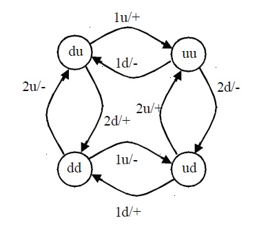
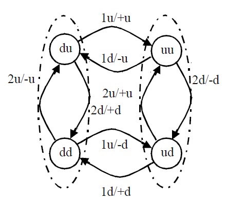
In the examples so far, every automaton state type corresponded to one and only one physical state type in a direct way, hence there was no need for a complex grouping of physical states types. Now, consider the physical system P₂ consisting of two switches Sw1 and Sw2 connected to a light bulb and a battery by a copper wire (as depicted in Figure 4). Input to P₂ consists in switching one of Sw1 or Sw2 from either “up” to “down” or vice versa. The four possible input states are, analogous to the previous notation, denoted by ‘1u,’ ‘1d,’ ‘2u,’ and ‘2d.’ The internal states of P₂ are the four possible states of the switches (denoted by ‘uu,’ ‘dd,’ ‘du,’ and ‘ud,’ where the first letter indicates the state of Sw1 and the second that of Sw2). Output of the system is again the state of the light bulb (denoted as before).

The abstract structure of P₂ for the above-defined input, inner, and output states, can be depicted as state-transition diagram, which also defines an automaton, call it M₂. The structure of this automaton is isomorphic to the causal structure of P₂ for the given physical states, hence, P₂ implements M₂.

Now suppose switch Sw2 is never pressed; then it can readily be seen that P₂ implements M₁, too. Starting in state “du,” the automaton can only transit between “du” and “uu”: ignoring Sw2 simply turns M₂ into M₁. Once Sw2 is used, however, there is no mapping that can relate the above-defined states in M₂ to states in M₁, since whether input “1u” turns the light on or off depends on the state of Sw2. We will sketch only part of the argument (since it is rather long and tedious given the number of possible mappings that one has to consider): take “du” to be the start state, which has to be set in correspondence with ‘A.’ Then either “1u” or “2d” or both have to be mapped onto ‘a,’ and as a consequence, either “uu” or “dd” or both will correspond to ‘B.’ Suppose we map “1u” to ‘a’ and “uu” to ‘B.’ Then “1d” has to correspond to ‘b.’ But this is not possible. To see this, suppose that “ud” will be mapped onto ‘A’ (since both, “ud” and “dd” must correspond to some automaton state). Then “2d” will have to correspond to ‘b,’ and consequently “1d” to ‘a.’ Contradiction. So, “ud” cannot be mapped onto ‘A,’ thus they must be mapped onto ‘B.’ But then, the transition “1d/+” turns the light on, as opposed to ‘b/0’ which turns the light off in M₁. So this is not possible either. Hence, “1d” cannot correspond to ‘b.’ It follows that “uu” cannot correspond to ‘B’ and “1u” not to ‘a.’ Thus, “2d” must correspond to ‘a,’ and so on…

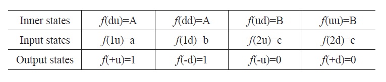
In the end, we establish that for the above-defined state types P₂ does not implement M₁. However, if other state types are considered, then there exists a mapping f under which P₂ implements the automaton M₁: take the output to be the state of the light bulb together with the state of Sw2 (resulting in the four distates “+u,” “-u,” “+d,” and “‑d,” where the first letter denotes the state of the light bulb and the second the state of Sw2). The idea here is to introduce extra output states so that the effect of pressing switch Sw2 can be ignored. This combination is physically legitimate, because all states are physically specifiable and support counterfactuals (it should thus be acceptable for Chalmers). In fact, every state will be acceptable as long as it can be specified within the physical theory that is used to describe the physical system (in this case circuit theory). Figure 6 depicts the causal structure of the two-switch system for the new states:

For the following, assume in addition that the input alphabet of M₁ contains the symbol ‘c’ (this does not change the automaton, since ‘c’ is not used in any transition in M₁—see also below). Define f to be the following function:

It can be seen that for “(A, a)→(B,1)” and “(B, b)→(A, 0)” (i.e., for every state transition) the conditional of Chalmers’ definition of implementation (i.e., “if the system were in state …, it would transit into …”) is true: take the first transition “(A, a)→(B, 1).” Two states of P₂ correspond to state ‘A,’ “du” and “dd.” Suppose P₂ were in state “du.” Since the only input corresponding to ‘a’ is “1u,” then P₂ would transit reliably into state “uu” (corresponding to ‘B’) and produce output “+u,” which corresponds to ‘1.’ Similarly, if the system were in state “dd,” then P₂ would transit reliably into state “ud” (corresponding to ‘B’) and produce output “-d” (corresponding to ‘1’). The same holds true for the second transition. Hence, according to Chalmers’ definition, P₂ implements M₁ under f (even if it does this in an admittedly strange way).

Together, we get that P₂ implements M₁ (under the above-defined function f) and P₂ also implements M₂ (which has a different, more complex transition structure than M₁). Assuming that automata are the appropriate formalism to reflect the causal structure of a physical system, one can reach two (not necessarily exclusive) conclusions: 1) physical systems can have multiple causal structures, which depend on the grouping of physical states (i.e., the level of description for a given set of physical states), or 2) Chalmers’ definition has to be modified to reflect the causal structure of the system determined by the given set of physical states.

The former does correspond to our intuition that the same physical system (i.e., the same spatio-temporal region) can be described at different levels according to different notions of physical state appropriate for that level. Note, however, that one is limited to groupings (that is, combinations) of the given physical states in the above case, which are, of course, limited to groupings that allow for reliable transitions between them.

The latter conclusion points in another direction: if computational descriptions are to “mirror” the causal structure of physical systems, then the causal topology of a set of physical states alone should be necessary and sufficient to specify the “corresponding” computational description. Although this approach does not leave any room for groupings of states into state types within the definition of implementation, it can still account for all of the potentially different computational descriptions obtained from Chalmer’s definition by simply considering the groupings of states (implicit in Chalmers’ definition) as states of a physical system (e.g., the same system at a different level of description). That way the second leaves open the possibility that physical systems might have more than one causal structure (depending on possible groupings of its states), while removing the burden from the theory of implementation to decide which of these groupings are legitimate and returning it to the theory that delivered these states in the first place (for an elaboration of this line of thinking, see Scheutz 2001).

1Example: “The automaton transits from state A to state B on input a producing output b” for the type and “After five inputs the automaton is in state A” for the token interpretation.  2A reason for this conceptual conflation might be that some physical systems might assume or instantiate any state (type) only at most once. For example, the construction in Putnam (1988) is essentially based on a physical principle that guarantees that (open) physical systems are always in different physical states at different times.

Unfortunately, Chalmers neither provides criteria for the formation of (basic) physical types nor for more abstract types, but is rather satisfied with the mere existence of a grouping of types into more complex types. In his second definition, he simply notes that his “[…] definition uses maximally specific physical states s rather than the grouped state-types” (Chalmers, 1994, p. 393). What exactly “maximally specific physical states” are is left open. Since time is left out in his definition, it must obviously enter here as part of the “physical state,” but it is not clear how. This too, makes it seem as if there need not be any resemblance between different physical states that can be grouped together to form a type as long as the function f maps them onto the same S_i, which opens doors to all kinds of wild implementations (aka Stabler).

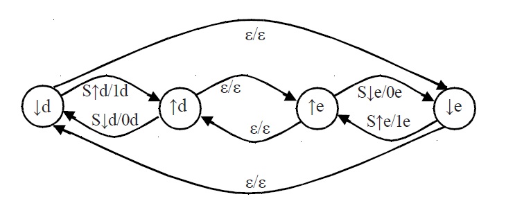
Consider system P₁, augmented by the temporal attributes “on weekdays” and “on weekends,” so that pushing the switch upwards/downwards on weekends can be distinguished from pushing it upwards/downwards on weekdays. The same distinction is made with respect to internal states: the switch can be in up/down position on weekdays and on weekends. Note that the system, call it P₁,₄, automatically changes states Fridays and Sundays at midnight, without further ado. The internal states of P₁,₄ are then “switch down on weekdays” (denoted by ‘↓d’), “switch up on weekdays” (denoted by ‘↑d’), “switch up on weekends” (denoted by ‘↑e’), and finally “switch down on weekends” (denoted by ‘↓e’). The time-dependent input states are “push Sw1 upwards on weekdays” (denoted by ‘S↑d’), “push Sw1 downwards on weekdays” (denoted by ‘S↓d’), “push Sw1 upwards on weekends” (denoted by ‘S↑e’), “push Sw1 downwards on weekends” (denoted by ‘S↓e’). The output states of P₁,₄ are denoted by ‘1d’ for “light on on weekdays,” ‘0d’ for “light off on weekdays,” ‘1e’ for “light on on weekends,” and ‘0e’ for “light off on weekends.” Figure 7 depicts the causal structure of P₁,₄ (note that the ε/ε-transitions account for the automatic change in states resulting from the influence of real-time):

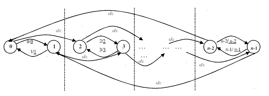
This construction can be generalized to allow a switch system P₁,_n to implement an arbitrary FSA (with m states, k different input and l different output symbols) by ensuring that P₁,_n has enough states and edges that can be mapped onto the graph of the FSA. The following theorem, christened the “Slicing Theorem” because it generates additional states by “cutting off temporal slices” of existing ones, states the requirements and its proof exhibits the construction:

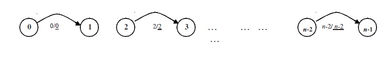
Proof: Consider the physical switch system with n=2k internal states (for k > 1) depicted as a graph with n nodes below. Each node is labeled with a (bold) natural number from 0 to n–1, and edges from node i to i+1 are labeled with i/i and edges from node i+1 to i are labeled with ‘i+1/i+1’ (e.g., the edge from node 3 to node 4 is labeled with ‘3/3’). There are ε/ ε-transitions from node i to i+2 (for i<n–2) as well as ε/ε-transitions from n–2 to 0 and from n–1 to 1. Each of the two original states of the switch system can be in k different states within an arbitrary given time interval I (e.g., if k=24, let I be one day and consequently consider switch states at each hour interval of the day).

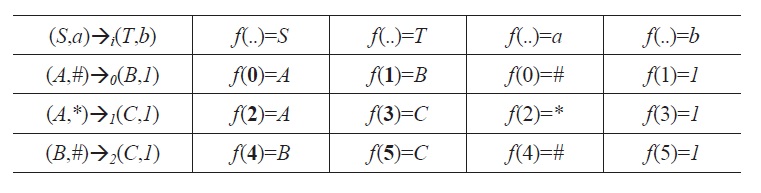
Pick an arbitrary FSA M with k transitions, input alphabet Σ and output alphabet Γ (where c∈Σ and d∈Γ are symbols that do not occur in any transition). Notice that M can have at most k+1 nodes (but must have at least one node).3 Without loss of generality, we can assume that the transitions are enumerated: →₀, →₁, …, →_k−1. Define the following mapping f for P₁,_n: for each transition (S, a)→_i(T, b) (where S, T are states and a∈Σ−{and b∈Γ−{d}) for i<k, let f(2i)=S, f(2i+1)=T, f(2i)=a, f(2i)=b, f(2i+1)=c, f(2i+1)=d (all transitions from 2i+1 to 2i are neglected). Then it can be checked that under this mapping P₁,_n implements M. The way this mapping works is simple: every transition of M is associated uniquely with a transition from node i to i+1

Thus, for every transition (S, a)→_i(T, b) in M, the following is true: if P₁,_n is in internal state 2i, it can only receive input 2i and produce output 2i (given the time-dependence of all inputs and outputs, 2i and 2i are the only states defined for that particular period of time, namely the time interval in which the switch system can be in states 2i and 2i+1—(*) other inputs/outputs that may be mapped onto a/b by f cannot be received/produced in that time period and need, therefore, not be taken into consideration). Given that P₁,_n is in internal state 2_i and receives input 2i (such that f(2i)=S and f(2i)=a), this reliably causes it to enter internal state 2i+1 and produce output 2i such that f(2i+1)=T and f(2i)=b.

There is an obvious weak spot in the above argument, marked by ‘(*).’ One could argue that even though other input/output states are not applicable (because they have been just so defined), they should not be excluded a priori, but be taken into consideration in the proof. In other words, if there are other inputs, even though they are not available at the respective state of the system, that are mapped onto a, say, then the definition of implementation should take care of them, but this is not the case. Take, for example, the following automaton:

Define f according to the above construction for the three transitions:

In checking whether the switch system so defined implements the automaton under f, one runs into the case where the switch system is in state 0 and receives the pendant to input ‘#,’ i.e., input 0 or input 4. Even though the latter is not possible if the system is in state 0, according to f, it maps onto input ‘#’ in the automaton, and is, thus, a legitimate candidate for an input. It follows that the antecedent of the conditional (in the definition of implementation) is (“theoretically”) true for internal state 0 and input 4, but that the consequent is false, because the system will not (reliably) transit into state 1 producing output 1. In fact, it will remain in state 0, because it did not receive any input in the first place. Hence, one could conclude that the theorem is not valid for cases such as the above.

Whether this kind of argument is valid or not, is left for the reader to decide. Even if the objection is correct and the theorem has to be restricted to cases where no two transitions use the same symbol, a strange aftertaste remains: the simple switch system will still implement a restricted, yet infinite class of automata. Besides: every language accepted by an automaton with k transitions without such a restriction can be obtained as a homomorphic image of the language of an automaton with k transitions with the restriction.

Before we discuss the consequences of the Slicing Theorem for general theories of implementation, note that this result can also be extended to CSAs, “which differ from FSAs only in that an internal state is specified not by a monadic label S, but by a vector [S¹, S², S³, …], where the ith component of the vector can take on a finite number of different values, or substates. […] Input and output vectors are always finite, but the internal state vectors can be either finite or infinite. The finite case is simpler, and is all that is required for practical purposes” (Chalmers, 1994, p. 394). We will, hence, assume internal states to be finite. The implementation conditions are then:

Chalmers points out that “a natural requirement for such a decomposition is that each element correspond to a distinct physical region within the system […] the same goes for the complex structure of inputs and outputs.” Again, he claims (wrongly) that “state-transition relations are isomorphic in the obvious way.” Furthermore, he is convinced that his CSA model prevents the notion of implementation from the threat of vacuity: “What counts is that a given system does not implement every computation […] This is what is required for a substantial foundation for AI and cognitive science, and it is what the account I have given provides” (1994, p. 397). This can be contrasted with the following theorem:

Theorem 5: [Extended Slicing Theorem] P_m,_2k implements any CSA with k transitions and m different substates of each state (for k>1 and m>0). Proof: Since the general proof is rather lengthy, but not difficult in principle, we will sketch it for a CSA M with 8 states which are vectors of three components (substates) that can each assume one of the two values ‘0’ and ‘1.’ M will read inputs which are vectors of two components and deliver outputs that are vectors of one component, both substates take values from {0, 1}.5 Since there are 4 possible inputs and 8 possible inner states (output states do not have to be counted separately, because whenever input and inner state are the same, the output has to be the same, too), M could have at most 4·8·8=256 transitions. We will show that P_3,256, a 3-switch system with three parallel switches/light bulbs connected to a battery and 256 internal states, implements M. First, consider the 3-switch system over some time interval Int, which is further divided into eight subintervals of equal length.6 The first switch can be in states on_Int1/2, off_Int1/2, on_Int2/2, off_Int2/2, the second in states on_Int1/4, off_Int1/4, on_Int2/4, off_Int2/4, on_Int3/4, off_Int3/4, on_Int4/4, off_Int4/4, the third in states on_Int1/8, off_Int1/8, on_Int2/8, and so on (“Int1/2” designates the first half, “Int1/4” the first quarter, “Int2/4” the second quarter, etc. of Int). Consider only transitions from “off” to “on” states. Then within Int, there are eight possible combinations of transitions for the three switches. Since there are also eight possible transitions between any two combinatorial states, one of the eight transitions can be mapped onto the one in M: if M transits between states [S₁, S₂, S₃] and [S₁’, S₂’, S₃’] on input [I₁, I₂] outputting [O₁], this corresponds to the 3-switch system transiting from state [off_IntX/2, off_IntY/4, off_IntZ/8] to state [on_IntX/2, on_IntY/4, on_IntZ/8] on input [a_Int, bc_Int] outputting [abc_Int] (where even values of the numerators X, Y, Z in the interval states correspond to the “0” value for automata substates, and those with odd values to the “1” value such that IntZ/8⊆IntY/4⊆IntX/2). The transition [1,1], [1,0,1]→[0,1,1], [0], for example, would correspond to [a_Intbc_Int], [off_Int2/2, off_Int3/4, off_Int6/8]→[on_Int1/2, on_Int2/4, on_Int4/8], [abc_Int]. Note that inputs and outputs of the automaton have to correspond to combined inputs and outputs (indicated by concatenating the respective characters) in the 3-switch system.

A physical state transition corresponding to a combinatorial state transition can then be defined as the transition taking place by pressing all 3 switches of the system during subinterval IntZ/8 of Int. Physical states are defined correspondingly for this interval, inputs and outputs are combined states of switches and light bulbs (as described above). The rest of the construction proceeds as in the construction of the Slicing Theorem (e.g., the division of the a cyclic interval I into k parts in order to account for k transitions—in the case of M 32 such parts are needed, since there are 4 four different inputs for each of the 8 possible combinatorial states; e.g., if the cyclic interval is one day, then the automaton could spend three quarters of an hour in one of the Int states). The main difference between the above construction and the previous one for the Slicing Theorem is that substates are mapped onto distinct spatial regions (i.e., the switches), and that the complex state transitions between substates is preserved. It follows, then, that P_3,256 implements M in the sense of Chalmers’ definition. As a consequence, generalizing the above construction, every CSA with at most m different substates of each combinatorial state is implemented by an m-switch system.

This kind of result that one physical system can implement “too many” computations is exactly what Chalmers tried to avoid when he proposed his definition against the background of Putnam’s construction showing that every ordinary open system implements every finite state automaton without input and output (Putnam 1988; see also Scheutz 1999). In a sense, the Slicing Theorems strengthens Putnam’s program against charges such as “wrong notion of causality,” “input/output missing,” “wrong level of description,” “unnatural physical types,” etc. All of these, except perhaps for the last one, are dismissed by the Slicing Theorems. This adds evidence to the claim that Putnam’s construction, as he notes at various places (e.g., Putnam, 1988, pp. 95), essentially points out the lack of appropriate state and type formation rules, and consequently contradicts Chalmers’ belief that physical states are not the main problem at hand: “there does not seem to be an objective distinction between ‘natural’ and ‘unnatural’ states that can do the relevant work. [⋯] I will not pursue this line, as I think the problems lies elsewhere” (Chalmers, 1996, p. 312). While Chalmers may be right that the distinction between “natural and unnatural states” does not do relevant work, his position that “the problem lies elsewhere” seems wrong given the results from the Slicing Theorems. Interestingly, the construction exploited in the Slicing Theorems differs in at least five crucial aspects from Putnam’s construction:

1) While Putnam’s construction shows how to implement a particular “run” of a computation, i.e., a particular sequence of state transitions, the above construction models the complete state-transitional structure of the automaton. That is why it only needs a finite (i.e., bounded) number of states to perform arbitrarily long computations (i.e., all possible computational sequences), whereas Putnam’s construction requires an unbounded number of states (depending on the length of the respective computational sequence). It exploits the fact that at some level of description physical configurations can be viewed as recurrent (whereas Putnam used the “Principle of Non-Cyclic Behavior” to obtain new physical states).7

2) Tokens of state types such as “switch up on Mondays” can be easily individuated (we can check if it is—currently or at some other time—Monday and we can check whether the switch is in position “up” or “down”). These input states have the predictive capacity that Putnam’s construction was criticized for; it is known ahead of time, what tokens of these types will look like and how they can be produced (as necessary requirement if one wants to control the input to a system!).

3) State transitions are reliable. Pressing switches is certainly as reliable an action as any reliable one can imagine (unless the switch is defective, etc., which can be accounted for by adding conditions of normal opera-tions to the definition of implementation as in the case of Definition 2). The same holds of the light bulbs being lit or not lit under the respective circumstances: given a setup corresponding to the wire diagram, the respective light bulbs will be lit reliably if the switches are in a position such that current can flow (and neither the battery, nor the wires, nor the light bulbs are defective). Transitions from one time interval into the next are obviously reliable as well, as they happen without further ado (and rely on the physical laws regarding the permanence of objects which are not subject to internal decay processes and/or external influences).

4) State transitions support counterfactuals. To see this, note that input occurs only “within time slices,” i.e., whenever a switch is pressed down on Monday, say, the system will reliably change state into “switch down on Monday.” If it is pushed up again, the system will return to state “switch up on Monday.” It can never be case that the system receives input on Monday and ends up in a state on Tuesday. Thus, any counterfactual of the form “had the system been in state p, on input in it would have transited into state q producing output out” is true for any time slice, and since input driven state changes cannot occur across time slices, it is vacuously true for those.

5) Because of the above and the laws of physics (i.e., circuit theory), the relevant state transitions (i.e., those that are input driven) are causal, not only according to a physical notion of causation, but to the stronger, counterfactual supporting notion that people like Chalmers and Chrisley, for example, require. It could be objected that temporal successions of one and the same physical state, i.e., state s at time t_n and state s at time t_n+1, cannot be said to be causal transitions. Granted! But this is true only of “irrelevant” state transitions (i.e., ε,ε-transitions). In automata theory, ε,ε-transitions are supposed to model transitions in a system that happen without further ado: no input is necessary, no output is produced, the automaton transits without input from one inner state to another—that is why this transitions are called ε,ε-transitions in the first place. The same is true of transitions between two time slices: no input is necessary, no output is produced, the system transits from one inner state into another without any external influence. In that sense these transitions are not caused by anything. That is why we limited the claim that state transitions are causal to relevant transitions, i.e., the ones that are causal. Only relevant transitions are mapped onto automata transitions, thus all transitions that are “mirrored” in the automaton are causal.

It seems that the only objection left to the above construction is the nature of the involved physical states, since the main charges (see Chalmers, 1996, or Chrisley, 1996) against Putnam’s Theorem that his notion of implementation is not based on reliable, counterfactual supporting, causal state transitions (i.e., that his notion of causality does not support counterfactuals) does not mutatis mudandis transfer to the Slicing Theorems. One conclusion to be drawn from the Slicing Theorems would be to disallow temporal individuations of physical states. That way one could savor Chalmers’ notion of implementation and explain what went awry in the above construction. This, however, seems to me too strong a restriction as there might be cases where temporality is crucial in individuating physical states: consider a shared memory between two processors such that the first processor accesses the memory during even clock cycles and the other during odd clock cycles. To understand what is going on in such a memory (e.g., when the value of a memory location has changed “between two successive states without further ado” from the perspective of one processor) one would probably introduce notions like “even state” and “odd” state to refer to states at certain clock cycles.

There is a better reply to the objection that the unwanted results of the Slicing Theorems result from temporally individuated states. Instead of individuating these states temporally, one could slightly modify the switch system by adding “a clock,” which reliably goes through a fixed cycle of physical states in a given amount of time (12·60·60 states per 12 hours, say). Then one can form the same “slices” that were used in the switch system to implement arbitrarily complex computations, except that the temporal individuation (the temporal slices) is now replaced by “spatial individuation” (of the clock hands, for example). By forming combined states such as “the switch at 5h34’33’ ” (where the time expression is used to fix a spatial position on the clock), the clock-switch system can implement very complex CSAs according to Chalmers’ definition of implementation using the construction of the Slicing (i.e., to be exact a one-switch system with one clock will implement any computation with up to 12·60·60 state transitions, and by adding additional clocks and/or increasing the number of distinct clock states, this number can be increased significantly). Yet, it is intuitively very clear that the system does not do any computational work.

3There could be more nodes, if some of them are unreachable from the start state. In that case, one needs to divide the time interval futher to obtain new states which can be mapped onto the unreachable ones, but this presents no difficulty  4I corrected the misprint in Chalmers’ article by substituting ‘k’ for ‘n.’  5For example, the CSA could compute the “carry” in an addition: it would take the input as binary number and add it to the number represented by the current state, then transit into a state which represents the sum (modulo 8) and report if a carry over has occurred during the addition (by outputting 1, otherwise 0). To illustrate this, assume the automaton is in state [1,0,1] and receives input [1,1]. This makes it transits into state [0,0,0] and with output [1]. Had it been in state [1,0,0], then the output would have been [0] and it would have transited to state [1,1,1].  6For k substates, each of which can assume any of n different values, one would have to consider nk different subintervals.  7Note that plausibility of the principle of non-cyclical behavior was one of the main points of attack of Putnam’s argument, see, for example, Chrisley (1994). Without this principle, Putnam’s construction cannot work.

The analysis of Chalmers’ definitions of implementation for FSAs and CSAs showed that they do not view computation as an abstract way of specifying the causal structure of a physical system such that “the formal state-transitional structure of the computation mirrors the causal statetransitional structure of the physical system” (Chalmers 1994, p. 393). For according to these definitions, physical systems do not implement only isomorphic computations for a given set of physical states and their causal relations, but rather many different (simpler) computations, which is what Chalmers must have intended when he wrote that “any system implementing some complex computation will simultaneously be implementing many simpler computations—not just 1-state and 2-state FSAs, but computations of some complexity” (Chalmers 1994, p. 397). Unfortunately, one cannot have it both ways: either “the relation between an implemented computation and an implementing system is one of isomorphism between the formal structure of the former and the causal structure of the latter” (Chalmers 1994, p. 396) or it is not (allowing for “simpler computations to be simultaneously implemented”).

If one were to go with the first alternative, then isomporphism might still be too strong a requirement, because there are infinitely many equivalent redundant computational descriptions of any given computational system that should all legitimately count as being isomorphic to the causal structure of the physical system. Hence, physical systems in that case would have to be viewed as implementing all computations that are bisimilar to their isomorphic computations (see Scheutz 2001 for details).

And if one were to go with the second alternative, it should not be the case that simpler computations which fail to capture and may even violate important parts of the causal structure of a physical system can be viewed as being implemented by that physical system (as is the case with Chalmers‘ definitions as shown by the switch system where the switch could be pressed only once). Moreover, the fact that even very simple physical systems can be viewed as implementing very complex computations (normally exhibited by very complex physical systems) under Chalmers’ definitions, contrary to what one would intuitively expect, points to a main deficiency in the Chalmers’ account: the lack of any constraints on physical state type formation. By replacing spatial complexity of physical states (in “complex” physical systems) with temporal complexity of physical states (in “simple” physical systems such as the switch systems), the two Slicing Theorems compensated lack of spatial structure by temporal structure and turned spatially structured causal patterns into temporally extended causal patterns. And using Chalmers’ own suggestion of adding a clock to a physical system in order to generate new physical states, one could turn non-effective temporal properties such as “the state of x on Monday” into effective spatial properties such as “the state of the all hands” on a certain clock (that way simple switch systems augmented by clocks could be even used for real computations). And if there were to be a worry about using the same clock state for individuating input, output and internal physical states, then one could add three clocks to the system for each state category.8

It is important to note that the Slicing Theorems do not only pose a threat to Chalmers’ definitions of implementation, but to any “(state-to-state) correspondence view of implementation” (CVI) as well as any “semantic view of implementation” (SVI) (e.g., Copeland 1996, Rappaport 1999), for that matter (just substitute “part of the system” for “state of the system”), precisely because both views crucially depend on a notion of “physical state” and/or “physical part.” CVI/SVIs need this notion to set up a correspondence between the physical and the abstract, yet the question of what counts as a legitimate physical state is not answered by any of them. CVI/SVIs can only provide an answer to the implementation problem for systems for which a set of physical states is given. If physical states are not given, CVI/SVIs run into insurmountable difficulties: following the construction of the Slicing Theorems, physical states supporting counterfactuals can be defined, for which the system implements almost any computation.

Two possible, non-exclusive conclusions are implied: computation is not the right kind of explanatory device for causal organizations of physical systems (and as a consequence for theories of mind), and/or CVI/SVIs are not the right kind of approach to a general theory of implementation (as they will fail as soon as a physical theory does not provide a well-defined notion of physical state). Note that CVI/SVIs are certainly applicable if physical states are given, which in real-world hardware design, for example, is obviously the case. Yet, the success of CVI/SVIs with systems that have been purposefully designed so as to allow for an easy state-to-state correspondence between physical states (which are given) and more abstract states should not distract from their failure in the general case (e.g., analog computers are a good example of designed devices that do not provide a clear-cut notion of physical state). Because computations have to be linked to concrete systems (which are described at a certain level) in order to be computations, the implementation relation must hold between computations and levels of descriptions of systems.

We are left with various questions unanswered: which (lower) level is the right one? Which level supplies the right kinds of states to be linked to the computational ones? Is there a systematic way to find the right level and find the right states/state types at this level? A theory of implementation should be able to answer all these questions in a systematic way for all possible levels of description. Any state-to-state correspondence or semantic view, however, is naturally limited to a level of description and a notion of state/part at that level and can, therefore, not provide any criterion for particular choices of levels. Furthermore, a theory of implementation should provide necessary and sufficient criteria to determine whether a class of computations is implemented by a class of physical systems (described at a given level), otherwise the term “implementation” is not appropriate. As long as these problems are not solved, we are back to square one (e.g., Kripke’s objections to the standard account of implementation) and constructions like the ones in the Slicing Theorems will continue to pose a threat to any CVI/SVIs.

8This worry was pointed out by an anonymous reviewer.