Object detection and recognition is becoming one of the major research areas in the field of computer vision. Feature points detection in images has become essential for several tasks in machine vision. Wide real-time applications can be found particularly in human-computer interaction, visual surveillance, robot navigation, and many more such fields. Further, feature points provide a sufficient constraint to compute image displacements reliably, and by processing these, the data are reduced by several orders of magnitude as compared to the original image data. These features could be shape, texture, colour, edge, corner, and blob.
The scale invariant feature transform (SIFT) algorithm extracts features that are invariant to image scaling and rotation, and partially invariant to changes in illumination and three-dimensional (3D) camera viewpoints [1]. They are well localized in both spatial and frequency domains, reducing the probability of disruption by occlusion, clutter, or noise. SIFT allows the correct matching of a single feature, with high probability, against a large database, which makes this algorithm highly distinctive, for providing a basis for object and scene recognition. Due to the emerging applications of keypoint matching-based object detection and the development of SIFT, a number of detection algorithms are focusing on invariant feature-based object detection. Some of the efficient object detection algorithms are Speeded Up Feature Transform (SuRF), Oriented Binary Robust Independent Elementary Features (ORB), and features from accelerated segment test (FAST) [2-4].
One of the most intuitive types of feature points is the
Object detection techniques detect the main points of an object in an image by dividing the image into three stages. The first stage examines the representation of features required for object recognition based on local or global image information. The second stage classifies the image based on the extracted features. The last stage is the recognition of the new image based on machine learning, which is performed by training images. The first step of object recognition is feature extraction that is used to detect the interest point of the image. The SIFT method is used to detect invariant feature points of an image.
>
A. Feature Detection Using SIFT
Lowe has demonstrated that SIFT features are invariant to image scaling, rotation, and translation, and partially invariant to changes in illumination and 3D viewpoints [1]. The following are the major stages of computation used to generate the set of image features:
1) Scale-Space Extrema Detection
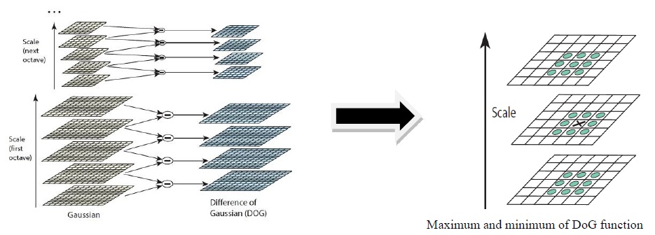
The first stage of keypoint detection is to identify locations and scales that can be repeatedly assigned under differing views of the same object. Detecting locations that are invariant to the scale change of the image can be accomplished by searching for stable features across all possible scales, using a continuous function of scale known as scale space [7]. The advantages of using this function are its computation efficiency and close approximation to the scale-normalized Laplacian of Gaussian, σ2∇2G [8]. For efficient detection of stable keypoint locations in the scale space, it has been proposed using the scale-space extrema in the DoG function convolved with the image, computed from the difference of two nearby scales separated by a constant multiplicative factor of ‘k’.
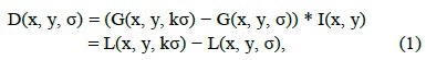
where
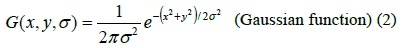

and I(x, y) is the image function.
2) Accurate Keypoint Localization
Once a keypoint candidate has been found by comparing a pixel to its neighbours (Fig. 1), a detailed model is fit to the nearby data for location, scale, and ratio of principal curvatures. According to the information obtained selected points that have low contrast (and are therefore sensitive to noise) or are poorly localized along an edge are rejected. Keypoints are selected on the basis of measures of their stability. A 3D quadratic function can be fitted to the local sample points to determine the interpolated location of the maximum that provides a substantial improvement to matching and stability [9]. For determining the location of the extremum, Taylor’s expansion of the scale-space function is utilized to derive an offset that sets the threshold of the extremum.
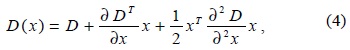
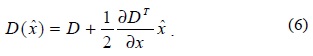
where D and its derivatives are evaluated at the sample point and x = (x, y, σ)T is the offset from this point. The location of the extremum, , is given by
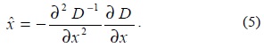
The function value at the extremum, D(), is useful for rejecting the unstable extrema with low contrast. This is shown as
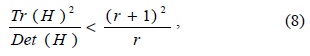
For stability, it is not sufficient to reject keypoints with low contrast. The difference-of-Gaussian (DoG) function will have a strong response along edges, even if the location along the edge is poorly determined and therefore unstable to small amounts of noise. To eliminate the principal curvature that is found to be lying mostly at the edges, a Hessian matrix is used for evaluation. The process of eliminating the edge response includes computing the Hessian and its trace and then, checking it with a threshold set by the ratio of the trace of Hessian and the product of its determinant, given by
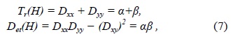
and the ratio given by

where r is the ratio between the largest magnitude eigenvalue (α) and the smaller one (β), so that α = rβ.
3) Orientation Assignment
Based on local image gradient directions, one or more orientations are assigned to each keypoint location. Due to this, the keypoint descriptor can be represented with respect to this orientation and therefore, achieve invariance to image rotation [1,10]. The scale of the keypoint is used to select the Gaussian smoothed image, L, with the closest scale, so that all computations are performed in a scale-invariant manner. For each image sample, L(x, y), at this scale, the gradient magnitude, m(x, y), and orientation, θ(x, y), are precomputed using pixel differences:
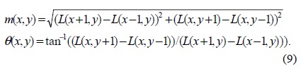
The gradient orientations of sample points that lie within a region around the keypoint form the orientation histogram. Prior to the addition to the histogram, each sample is weighted by its gradient magnitude and by a Gaussianweighted circular window when σ is 1.5 times that of the scale of the keypoint.
4) Keypoint Descriptor
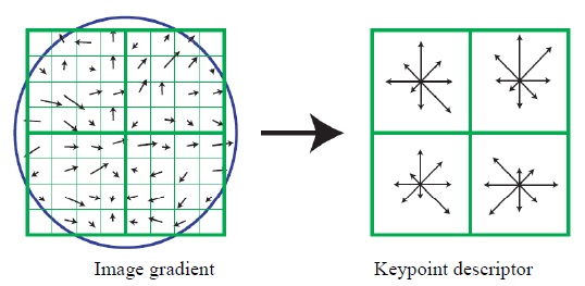
The local image gradients are measured at the selected scale in the region around each keypoint. These are transformed into a representation that allows for significant levels of local shape distortion and changes in illumination.
A descriptor is computed for the local image region that is highly distinctive yet is as invariant as possible to the remaining variations, such as changes in illumination or 3D viewpoints. A complex cell model approach based on a model of biological vision [11] provided better matching and recognition than a traditional correlation of image gradients. A keypoint descriptor is created by computing the gradient magnitude and orientation at each image sample point in a region around the keypoint location (Fig. 2). These are weighted by a Gaussian window with σ equal to one half of the width of the descriptor window, shown as a circle. The orientation histograms accumulate these samples, summarizing the contents over 4 × 4 sub-regions, with the length of each arrow corresponding to the sum of the gradient magnitudes in that direction within the region.
Finally, the feature vector is modified to reduce the effects of illumination change. The descriptor is invariant to affine changes in illumination.
In the application to object recognition in presence of occlusion and clutter, clusters of at least three features are required. This procedure involves three stages:
>
B. Feature Detection Using FAST
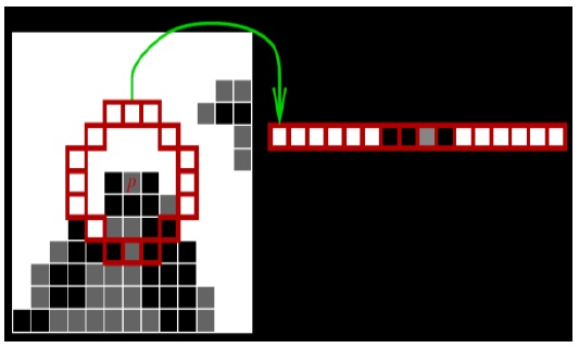
FAST is used for high-speed corner detection. The segment test criterion operates by considering a circle of sixteen pixels around the corner candidate ‘p’, as shown in Fig. 3.
The detailed algorithm is explained below:
Although the detector exhibits high performance in itself, there are a few limitations. First, this high-speed test does not reject as many candidates for n < 12, since the point can be a corner if only two out of the four pixels are significantly brighter and darker than
1) Improving Generality and Speed With Machine Learning
The process operates in two stages. First, a set of images is taken for training. To build a corner detector for a given n, all of the 16 pixel rings are extracted from the set of images. In every image, run the FAST algorithm to detect the interest points by taking one pixel at a time and evaluating all the 16 pixels in the circle. For every pixel ‘
For each location on the circle x ∈ {1 . . . 16}, the pixel at this position with respect to
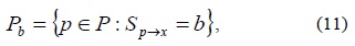
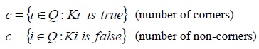
Let P be the set of all pixels in all training images. Choosing an x partitions P into three subsets, Pd, Ps, and Pb, where

and Pd and Ps are defined similarly.
Let Kp be a Boolean variable which is true if
The total entropy of K for an arbitrary set of corners, Q, is

where
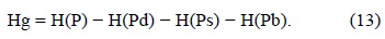
The choice of x then yields the information gain (Hg):
After selecting the x which yields the most information, the process of entropy minimization is applied recursively on all three subsets, i.e. xb is selected to partition Pb into Pb,d, Pb,s, and Pb,b ; xs is selected to partition Ps into Ps,d, Ps,s, and Ps,b ; and so on, where each x is chosen to yield maximum information about the set to which it is applied. The process is terminated when the entropy of a subset becomes zero. For a faster detection in other images, the order of querying which is learned by the decision tree can be used.
2) Non-maximal Suppression
Since the data contain incomplete coverage of all possible corners, the learned detector cannot detect multiple interest points. To ensure detection exactly similar to the segment test criterion in the case of FAST-n detectors, an instance of every possible combination of pixels with low weight is included. Non-maximal suppression cannot be applied directly to the resulting features as the segment test does not compute a corner response function. For a given n, as the threshold is increased, the number of detected corners will decrease. The corner strength T is defined as the maximum value for which a point is detected as a corner. The decision tree classifier can efficiently determine the class of a pixel for a given value of T. The class of a pixel (for example, 1 for a corner, 0 for a non-corner) is a monotonically decreasing function of T. Therefore, we can use bisection to efficiently find the point where the function changes from 1 to 0. This point gives us the largest value of T for which the point is detected as a corner. Since T is discrete, this is the binary search algorithm.
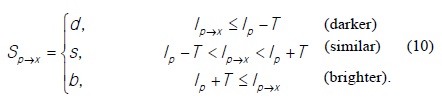
Alternatively, an iteration scheme can be used. A score function V is computed for each of the detected points (using midpoint circle algorithm). The score function can be defined as ‘the sum of the absolute difference between the pixels in the contiguous arc and the centre pixel’. The V values of two adjacent interest points are compared, and the one with the lower V value is discarded. Mathematically, this can be represented as
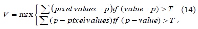
where
The score function can also be defined in alternative ways. The keypoint here is to define a heuristic function which can compare two adjacent detected corners and eliminate the comparatively insignificant one. The speed depends strongly on the learned tree and the specific processor architecture. Non-maximal suppression is performed in a 3 × 3 mask.
III. EXPERIMENTAL RESULTS AND DISCUSSION
Experiments using SIFT and FAST algorithms were carried out by taking a sample image in greyscale using the MATLAB R13b computer vision tool.
The SIFT features were extracted and plotted on the image so as to get a detailed view of the keypoints. The SIFT algorithm is derived from its descriptors. Hence, the total time calculated for the extraction of features is based on the time of descriptor calculation. Fig. 5 shows the keypoints extracted from an image by applying the SIFT algorithm. Table 1 shows the simulation result parameters, such as the time required for the calculation of keypoints and descriptors, intensity variation, rotation by angle, and different values of sigma. We have used σ = 1.6 which provides optimal repeatability and maximum efficiency in terms of image matching. The larger the number of keypoints matched, the more efficient will be the object recognition.
[Table 1.] Parameters obtained from scale invariant feature transform (SIFT) algorithm
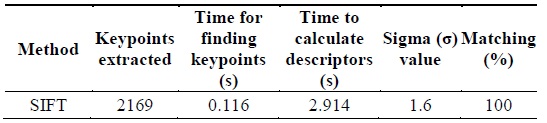
Parameters obtained from scale invariant feature transform (SIFT) algorithm
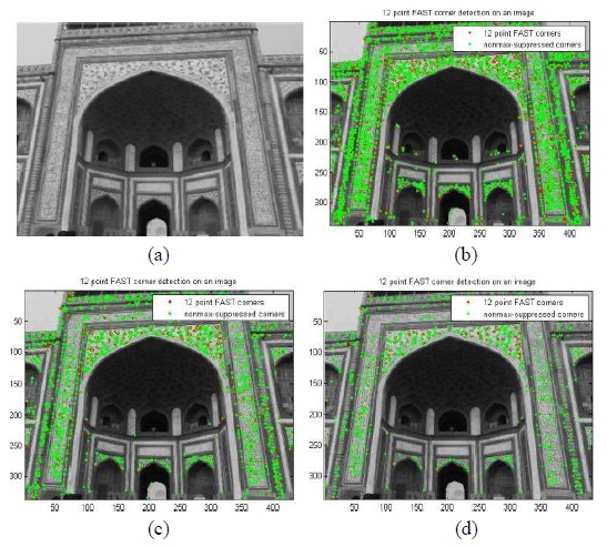
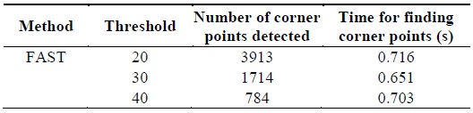
A machine learning algorithm was employed in a FAST-12 detector which detected corner points with a higher speed and repeatability. A non-maximal suppression algorithm is applied to the detector to remove the adjacent corners. The simulation result shows (Fig. 6) that the FAST-12 detector has dramatic improvements in repeatability over FAST-9 in noisy images. We focused our attention to optimize the detector for computational efficiency and make it more useful for real-time applications such as object recognition.
The figure was obtained with different threshold values and was observed that the number of corner points detected varied in accordance with the threshold set as shown in Table 2. From Table 2, it is found that at a threshold of 30, the corner points are detected in the image with less computational time than the threshold values of 20 and 40.
[Table 2.] Parameters obtained from features from accelerated segment test (FAST) algorithm

Parameters obtained from features from accelerated segment test (FAST) algorithm
IV. CONCLUSION AND FUTURE WORK
In this study, we analysed and compared the results of SIFT and FAST detector algorithms for object detection based on corner and feature points with respect to efficiency, quality, and robustness. The overall performance shows that although SIFT keypoints are useful because of their distinctiveness, the FAST algorithm has the best average performance with respect to speed, number of keypoints, and repeatability error. This property of SIFT features enables correct matching for a keypoint with other keypoints from a large database. Therefore, the SIFT algorithm has better performance in object detection although it is not improved for real-time applications. However, the machine learning approach used in FAST makes the algorithm faster in computation which adds to improvement in video quality, unlike other algorithms. FAST could achieve real-time performance in the object detection in an embedded device with increased speed. However, the overall performance of FAST for object detection is not significantly high as compared to other object detection methods because this algorithm is a little insensitive to orientation and illumination changes. Therefore, it is concluded that the FAST algorithm performs better with higher computational speed and is suitable for real-time applications. Future work in this area will focus on modifying the FAST algorithm for better feature detection with accurate orientation and responsive to changes in illumination while maintaining the processing speed.


![Image showing the interest point under test and the 16 pixels on the circle (image copied from [5]).](http://oak.go.kr/repository/journal/17409/E1ICAW_2014_v12n4_263_f003.jpg)
![Vector showing the 16 values surrounding the pixel p (*image copied from [6]).](http://oak.go.kr/repository/journal/17409/E1ICAW_2014_v12n4_263_f004.jpg)