System identification is a very important issue in system engineering. In recent decades, neural networks [1-3] and fuzzy systems [4-7] are often used to model complicated systems. In these modeling approaches, the task is to obtain a set of fuzzy rules or a neural network that can overall act like the system to be modeled. These approaches can construct systems directly from the input-output relationship without the use of any domain knowledge. Thus, they are often referred to as model-free estimators [1]. Neural fuzzy system (NFS) [8-10] is basically a fuzzy system that has been equipped with learning capability adapted from the learning idea used in neural networks. Due to their outstanding system modeling capability, NFS have been widely employed in various applications. Basically, the main concern of NFS is learning. As mentioned, NFS is a model-free estimator. Thus, it is natural to consider learning as the main issue for system performance. In fact, the structure used to learn may also bring significant differences for those approaches. This can be seen from [11, 12] about the comparison of fuzzy systems and neural networks. In this article, we intend to discuss several ideas regarding the learning of NFS for modeling systems.
The first issue discussed here is about structure learning techniques. It is easy to see that when the number of input variables or the number of fuzzy sets for a variable increase the fuzzy rule numbers will exponentially increase. But, usually, meaningful data patterns do not spread out in the whole region. Thus, it is not necessary to use all possible rules in the system for learning. Then to define which rules should be used can be conducted through the so-called self-organization process. This process is usually referred to as the structure learning stage. It is to define rules from data. Such an idea is first proposed in [13] and later on, various approaches were proposed. Those ideas are introduced in this article.
The second issue is about the use of recurrent networks in NFS to model dynamic systems. This kind of approach is often called recurrent NFS or RNFS in the literature. Recurrent networks are those networks of which the inputs of some nodes are from following layers so that it forms loops. RNFS is to have feedback links from some layers to some nodes (usually are input nodes). In this approach, the feedback links are with delay and it can be found that in this case, there is no signal chasing phenomenon as expected for recurrent networks. Thus, RNFS does not have various problems considered in recurrent networks, like stability. To distinguish this difference, in our study, it is referred to as delay feedback NFS instead of recurrent NFS. In this article, the discussion about the performance of such systems will be given. It can be found [14] that such a delay feedback can only bring one order to the system not all possible order as claimed in the literature.
Finally, we will consider the use of the issue of using recursive least square (RLS) algorithms for the learning of fuzzy rule consequences and the rule correlation effects in NFS. Usually the consequence parts of NFS are characterized by singletons or linear functions [13, 15, 16]. When linear functions are considered, two different kinds of update rules, Backpropagation (BP) and RLS algorithms can be used for updating those parameters. The BP algorithm is adapted from the learning concept of neural network [11, 17] and is easy to implement. In BP, the current gradient, which can be viewed as the local information is used to update parameters. Thus, BP algorithm may suffer from low convergence speed and/or being trapped in local minima. On the other hand, adaptive neuron-fuzzy inference system (ANFIS) [15] and self constructing neural fuzzy inference network (SONFIN) [13] are to use the RLS algorithm originally proposed in [16] in the learning process. However, in practical applications, there are problems and then various remedy mechanisms may be needed while using RLS for the learning process in NFS. We have analyzed the effects of those approaches in our previous work [18, 19]. In this article, the interaction between rules on consequent part and RLS algorithm will be analyzed. Furthermore, the operation of resetting the covariance matrix is also discussed.
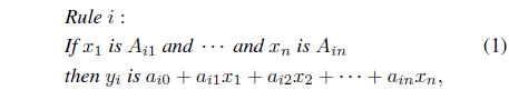
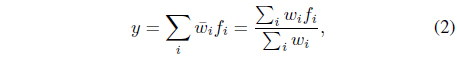
NFS have been widely used in last two decades. ANFIS [15] is the most-often mentioned NFS. In the learning phase, ANFIS uses all possible combinations of fuzzy sets in defining rules and it can be expected that some rules may be useless. As being equipped with structure learning capability, the SONFIN is proposed in [13]. The structure of SONFIN is created dynamically in the learning process and the system only uses rules that are necessary. For the other parts, there is no different between SONFIN and ANFIS. They are to realize a fuzzy model of the following form:

where
where
In the learning phase of SONFIN, rules are created dynamically as learning proceeds upon receiving training data. Three learning processes are conducted simultaneously in SONFIN to define both the premise and consequent structure identification of a fuzzy if-then rule. They are (A) input/output space partitioning, (B) construction of fuzzy rules, and (C) parameter identification. Processes A and B serve as the structure learning, and process C belongs to the parameter learning phase. In the structure learning phase, when a new fuzzy set is needed, its width (variance) can be defined by different initial values. When a small value is considered, it can be regarded as using the linguistic hedge “very.” This kind of discussion about fuzzy membership functions is given in [20], in which different parameter identification methods are considered and discussed. The learning process (A) is to partition the input space based on the input data distribution. In the process, when the current existing rules of the system cannot sufficiently cover the new input pattern, the system will created a new rule from this input pattern. To sufficiently cover means the current input pattern cannot have a sufficiently large firing strength from all existing rules. This firing strength threshold will decide the number of input and output clusters generated in the SONFIN and in turn will determine the number of rules used in the system. In other words, this threshold will define the complexity of the system. However, as reported in our previous work [20], different thresholds (or different variances) affect not only the complexity of the system, but also the performance of the RLS algorithm. In this study, the correlation terms in the covariance matrix used in the RLS algorithm will be studied. As mentioned, the dimension of the RLS algorithm covariance matrix is [(input number+1)×(rule number)]2. An obvious disadvantage of using RLS is the computational burden when the input number and/or the rule number are large. This is the reason that some approaches may tune the consequence parameters by assuming those rules are independent [13]. But our study shows that such ignorance of the correlation terms may degrade the learning performance. We will further discuss this issue in the next section. After a new rule is generated, the learning process (B) is to define fuzzy rules based on the current input data. The process is straightforward and the details can be found in [13].
Finally, the parameter-identification process is done concurrently with the structure identification process. For simplicity, a single-output case is considered here. The goal is to minimize the cost function , where

where
As mentioned, in SONFIN, the parameters of the premise part (i.e., those means (
In this section, several self-organization learning ideas used in the structure leaning for of NFS will be introduced. As mentioned, it is not necessary to use all possible rules in the system for learning. To construct a fuzzy model, the fuzzy subspaces required for defining fuzzy partitions in premise parts and the parameters required for defining functions in consequent parts must both be obtained. In the original Takagi-Sugeno-Kang (TSK) modeling approach [16], users must define fuzzy subspaces in advance, and then, the parameters in consequences are obtained through the RLS algorithm. This simple idea is then employed in ANFIS [15]. It can be found that those approaches must use all possible rules. In the following, we shall discuss ways of defining rules.
As mentioned in the above section, in the learning phase of SONFIN [13], rules are created dynamically as learning proceeds upon receiving training data. Three learning processes are conducted simultaneously in SONFIN to define both the premise and consequent structure identification of a fuzzy if-then rule. This kind of learning approach is somehow said to be an online learning approach. In that approach, even though in this structure learning phase, the process can be on line, the later learning algorithm, like BP is not suitable for online learning due to slow convergent property of the BP learning algorithm, which usually needs hundreds or thousands of epochs to converge. This effect can be seen from [23] that even a simple direct-generation-from-data approach [6] can outperform SONFIN in an online learning situation. Thus, it can be found that various structure learning approaches that are not online approaches were proposed in the later studies.
A simple idea is to use the original structure learning in [17]. In that approach, the input space is first divided into fuzzy subspaces through a clustering algorithm called the Kohonen self-organized network [24] according to only the input portion of training data. It can be found that the obtained fuzzy subspaces may not cover the entire input space. Note that this approach is similar to that in SONFIN and the fuzzy partition is only based on input data. In other words, rules are defined only based on the distribution of input portion of training data. Usually, in the literature, this structure learning stage is called the coarse tuning stage. After the fuzzy subspaces are defined, the system is approximated in each subspace by a linear function, through supervised learning algorithms, such as BP or least-square learning algorithms [2, 6, 7, 11]. In the meantime, the fuzzy subspaces may also be tuned usually through BP learning algorithms. This stage is called the fine tuning stage. Note that each subspace corresponding to one fuzzy rule is supposed to have a simple geometry in the input-output space, normally having the shape of ellipsoid [25]. In fact, other fuzzy clustering algorithms, such as the fuzzy C-mean (FCM) [26, 27] are also suitable to define fuzzy subspaces for fuzzy modeling. In general, the above mentioned approaches partition fuzzy subspaces based on only the clustering in the input space of training data and do not consider whether the output portion of the training data supports such clustering or not. In other words, such approaches do not account for the interaction between input and output variables.
Similar to the use of the AND operation in the fuzzy reasoning process, the match of a rule for a data set requires that the input portion and the output portions must be both matched with the premise part and the consequence part of the rule. Thus, to construct a rule, the input data and the output data must be both considered. Hence, the authors in [25, 27] considered the product space of input and output variables instead of only the input space in classical clustering algorithms for fuzzy modeling. However, these approaches and the above approaches still define fuzzy subspaces in a clustering manner and do not take into account the functional properties in TSK fuzzy models. In other words, in those approaches, training data that are close enough instead of having a similar function behavior are said to be in the same fuzzy subspace. Thus, if the consequence part is a fuzzy singleton, it is nice. But, if the consequence part is a linear function as usual be, such a structure learning behavior may not be proper. As a result, the number of fuzzy subspaces may tend to be more than enough.
In order to account for the linear function property, another approach is proposed in [28]. In the approach, fuzzy subspaces and the functions in consequent parts are simultaneously identified through the use of the fuzzy C-regression model (FCRM) clustering algorithm. Thus, not like to calculate a distance to a point (cluster center) in clustering algorithms, the approach is to calculate the distance to a line in a linear regression approach. This distance is then used to define an error function used in the cost function. The idea of this kind of approaches is to find a set of training data whose input-output relationship is somehow a linear function, and then, those training data can be clustered into one fuzzy subspace. Similar to other approaches, the structure learning behavior does not incorporate the optimization process in modeling and hence, the fine tuning stage supervised learning algorithms can further be used to adjust the model.
It should be note that in the above clustering or regression algorithms, users must assign the cluster number, which is supposed to be unknown. Another idea proposed in [29] is to employ the so-called robust competitive agglomeration (RCA) clustering algorithm used in computer vision and pattern recognition [30] to form subspace. In this approach, the cluster number is determined in the clustering process. Besides, the clustering process begins from the whole data set and then can reduce the effects of data sequence. As a result, it can have fast convergent speed and better performance as claimed in the literature.
Another consideration is about outliers in training data. The intuitive definition of an outlier [31] is “
4. Delay Feedback and Dynamic Modeling
It can be easily found that NFS can only model static system due to no memory in keeping previous states. When a dynamic system is the modeling target, an often-used approach is to use all necessary past inputs and outputs of the system as explicit inputs. Such a structure is referred to as the nonlinear autoregressive with exogenous inputs (NARX) model [14, 46]. Another kind of approaches [14, 47-49] is to feedback the outputs of internal nodes in networks with a time delay. Those methods have shown to have nice modeling accuracy on modeling dynamical systems in some examples. Such networks are usually called recurrent networks in the literature [47-49]. However, it can be found that even though the system indeed have loop in the connections, the feedback is with a time delay and then the system does not have actual loop. Thus, in our study, it is called the delay feedback networks [14].
Delay feedback networks are to use internal memories to catch internal states. We can also introduce delay feedbacks to account for dynamical behaviors in SONFIN. However, where to put those delay links is not so straightforward because there are semantics associated with those layers. Different from that used in [47, 48], another delay feedback approach for SONFIN, termed as the additive delay feedback neural fuzzy network (ADFNFN) is proposed in [14]. The basic idea is to adopt the autoregression and moving-average (ARMA) type [50] of modeling approaches. In an ARMA model, the output is predicted as a linear combination of the current input and previous inputs and outputs. In other words, previous outputs are included into the prediction model in an additive manner. In fact, NARX models can generally be viewed as a nonlinear extension of ARMA models because they mix all inputs in an additive manner (linear integration functions in neural networks and linear consequence functions in SONFIN). From simulations, it is evident that the proposed ADFNFN can have better learning performances than those approaches proposed in [47] and in [48] do.
It is noted that the prediction for the next step in dynamic systems is always based on previous data for a series-parallel identification scheme [50]. Then, when the step size is small, the possible error generated in one step will also be small. This correspondence will make the traditional root mean square errors (RMSE) not able to truly capture the ideas about how accurate the current model can predict. Another evaluating index called the non-dimensional error index (NDEI) is considered in [51] to evaluate modeling errors. The NDEI is defined as:
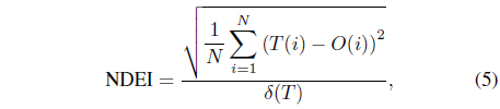
where
[Table 1.] Learning errors (RMSE) for Sinc with change algorithms
Learning errors (RMSE) for Sinc with change algorithms
Intuitively, the use of delay feedback could model any order of dynamic systems because those delay elements can be al kind of signals including those delayed ones. However, from [14], it can be found that those delay feedback models can only achieve the accuracy level of order-2 NARX models. In other words, those delay feedback networks seem not able to model the systems as accurately as the NARX models with proper orders do. It is because delay feedback models only use one delay in the modeling approaches, it is somewhat similar to NARX models with order 2. As shown in [14], if two feedback connections are used for each internal state; one is with one delay and the other is with two delays, it can be found that the errors have been significantly reduced when the considered systems are order-3 and order-4 systems. However, the modeling accuracy for the order-4 system is still not good enough. It is clearly evident that the role of the used delay number in a delay feedback model is similar to that of the system order in an NARX model. Thus, it can be concluded that delay feedback network is not necessary because it is more complicated than an NARX model with a proper order and cannot provide better performance.
As mentioned, ANFIS [15] and SONFIN [13] employ the RLS algorithm originally proposed in [16] in the learning process. However, in practical applications, there are problems and then various remedy mechanisms may be needed while using RLS for the learning process in NFS. In this article, the interaction between rules on consequent part and RLS algorithm will be analyzed and the operation of resetting the covariance matrix is also discussed. In the literature, RLS algorithms have been widely used in adaptive filtering, self-tuning control systems and system identification [53]. From the literature, it can be found that there are several advantages in using RLS algorithms, such as fast convergence speed and small estimation errors, especially while the system considered is simple and time invariant. Theoretically, the estimation of RLS is the best estimation under the assumption of Gaussian noise in ideal cases. In practical applications, there are some possible remedies. The advantage of those approaches can be obviously but not always while the system considered becomes complicated. Recently, IRSFNN [49] also present two types of parameter identification steps, which we referred to as the reduced and full covariance matrices for RLS algorithms. To explain the results in [49], the overlap coefficient is employed to define the intersection between fuzzy sets. Similarly in our previous work [20], two types of membership functions are considered to manifest what the differences between full and reduce covariance matrix are. When the system has more interaction between fuzzy sets, it can be found that the off-diagonal parts of the covariance matrix should not be ignored.
In our study, SONFIN [13] is employed as the NFS. In this section, the learning algorithms used in the original SONFIN are considered as a basis. The structure of SONFIN is created dynamically in the learning process and only uses rules that are necessary. It is easy to see that SONFIN can have very nice performance especially when the number of input variables is large. In the learning process, when the firing strength of the current input feature is lower than a threshold, the system will generate a new fuzzy rule for this input feature. In other words, if necessary, SONFIN can generate new fuzzy rules for new input features. After constructing fuzzy rules, the parameters of the premise part and of the consequent part of the NFS are updated through BP and RLS, respectively. It can be found that there are two kinds of interactions; interaction between input data and interaction between consequent structures. In order to have the efficient computation, the consequence parameters of SONFIN are calculated independently among rules [13]. However, it is expected that with the consideration of those rule interactions, it can help in discovering new knowledge among rules and improving the reasoning accuracy [13]. If the membership functions are of less overlapping, no matter what kinds of RLS algorithms are used, there is no much difference in the learning performance [20].
As mentioned in [54-56], those pre-defined membership functions can be modified (or tuned) by some operations, like “very” or “more-or-less”. When membership functions are tuned, linguistic variables can bring more human-like thinking with different kinds of membership functions. In SONFIN, the system also has the capability of changing the cores and shapes of membership functions. Consequently, SONFIN can have nice performance in data learning. However, those tuning effects may destroy original features of those membership functions. Since SONFIN only creates rules that are necessary, those original membership functions may contain some characteristics for that data pair. While the membership functions are tuned in the later learning process, those characteristics may be altered and more complex interactions emerge. As mentioned in [57], redundancy interaction usually cannot have significant improvement in performance. Besides, the correlation terms in the covariance matrix required in RLS is another problem. When the dimension of the system to be modeled becomes very large, the computational time required may become infeasible because of the dimension of the covariance matrix is (the number of rules×the number of input variable+1)2. Also, the interaction between BP (used for the tuning of input fuzzy membership functions) and RLS (used for the tuning of the consequence parameters) will be unexpected. In this study, the interaction between rules on consequent part and RLS algorithm will be analyzed and the operation of resetting the covariance matrix is also discussed.
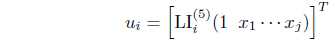
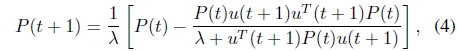
In this section, we will rearrange the analysis in [20] to analyze the performance of using the RLS algorithm with the full covariance matrix and with a reduced covariance matrix. The RLS algorithm with the full covariance matrix is the original approach as Eqs. (3) and (4) where
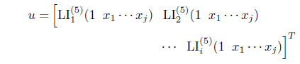
where is the firing strength of the ith rule and the supscript (5) means it is on the layer 5 of the whole structure [13]. For the reduced matrix case, the consequence parameters among rules are assumed to be independent. Thus, for Eq. (3), the input vector of u for the ith rule is

Then the covariance matrix
In [57], three kinds of interaction for sensory inputs are defined. They are
SONFIN updates the membership function and consequent parts simultaneously in the learning process. Interaction in each rule is difficult to manipulate. When BP changes the membership function and the consequent part change by RLS algorithm in one step, new membership functions will change the Layer 5 input, which makes the premise part used in previous RLS calculation changed. Somehow such a change can be viewed as the system is time varying. Thus, there are several methods proposed in the literature to resolve this problem, like to use a forgetting factor in the RLS algorithm, to reduce the learning constant in BP.
Another issue in the use of forgetting factor in the RLS algorithm is about resetting the covariance matrix P. It can be found that resetting the covariance matrix can somehow improve the training performance from our previous study [18]. However the overfitting phenomenon may occur in some cases. By setting the covariance matrix with a large diagonal values, the RLS algorithm will have the capability to focus on the present data. It is called bootstrap [58]. In other words, we set the system turn into local learning phase to reduce the effect from previous learning.
Two functions are considered for illustration for this part of study. First, a simply function
We continue the simulations in [19]. In the case of
[Table 2.] Learning errors (RMSE) for Sinc
Learning errors (RMSE) for Sinc
[Table 3.] Learning errors (RMSE) for Sinc with reset

Learning errors (RMSE) for Sinc with reset
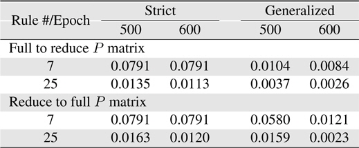
While the rule system is of generalized rules cases and the interaction among rules are significant, the original (Full) covariance matrix must be used. However, it can be expected that when the full matrix is considered in the RLS algorithm, the computation problem owing to a large dimension of the covariance matrix may be there. In order to have a better computational efficiency, the learning can use different RLS algorithms after resetting the
The second simulation is the identification of the
[Table 4.] Learning errors (RMSE) for Macky-Glass

Learning errors (RMSE) for Macky-Glass
[Table 5.] Learning errors (RMSE) for Macky-Glass with reset
Learning errors (RMSE) for Macky-Glass with reset
[Table 6.] Learning errors (RMSE) for Macky-Glass with change algorithm

Learning errors (RMSE) for Macky-Glass with change algorithm
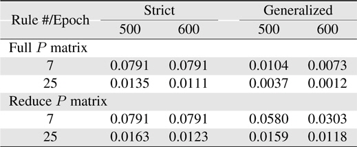
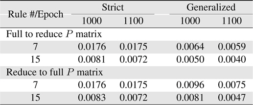
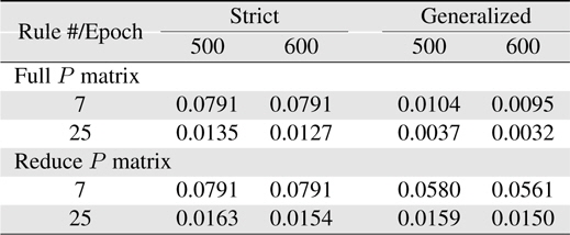
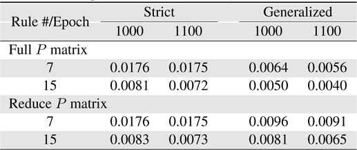
Now, more complexity for the Macky-Glass function is considered. In [49], four past values are used for training. 1000 patterns are generated in this study. First 500 patterns are used for training and the other 500 patterns are reserved for testing. After 100 epochs, the error for the generalized system with the use of full matrix is significantly better than others. In other words, most researchers recommend to use the reduce covariance matrix to save computational burden, it can be found that the error difference is not slight. In practice, the change of using different covariance matrices after resetting can be employed to improve learning performance. In this study, the covariance matrix is reset to the initial status at 10 epochs. The results are shown in Table 7. Comparing the performance between resetting and non-resetting, two cases become worse; strict rules with full covariance matrix system and generalized rules with reduce covariance matrix system. Some approached are considered here. First, the initial value of the covariance matrix diagonal parts is reduced to increase the effects from previous learning. The simulation results are shown in Table 8. Secondly, we reset the system with the full covariance matrix and the simulation result shown in Table 9.
[Table 7.] Learning errors (RMSE) for 4-input Macky-Glass with reset after 10 epochs

Learning errors (RMSE) for 4-input Macky-Glass with reset after 10 epochs
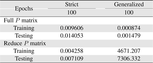
Learning errors (RMSE) for 4-input Macky-Glass with reset and reduce the covariance matrix diagonal values from 1000 to 1
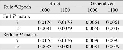
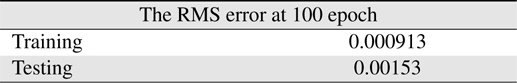
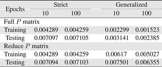
[Table 9.] Learning errors (RMSE) for 4-input Macky-Glass with full covariance matrix reset

Learning errors (RMSE) for 4-input Macky-Glass with full covariance matrix reset
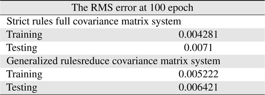
From those results, it can be found that in this case only resetting the covariance matrix is not enough to improve the learning performance. In Table 8, the learning performance at 100 epochs 0.004281 is better than that in Table 7. Also for generalized rules with reduce covariance matrix system case, to reduce the value of covariance matrix diagonal parts can indeed prevent the system unstable so as to catch up with the generalized rules with the reduce covariance matrix system results in Table 10.
[Table 10.] Learning errors (RMSE) for 4-input Macky-Glass
Learning errors (RMSE) for 4-input Macky-Glass
NFS is a nice modeling technique. In this article, we make a brief survey about its use in various aspects. For the structure learning, from the basic idea used in the original approach to the several different approaches are introduced. Hopefully, readers can understand those ideas and can select a suitable approach for their applications. For the dynamic system modelling, the idea of recurrent network, which has been widely used in the literature, is discussed. From the results reported in [14], it is clearly evident that such a methodology is not a good approach even though lots of researchers have used this idea in their approaches. A simple approach use a sufficient order in a traditional NARX model will have the best results. Finally, the effects on rule interaction in the use or RLS are reported in this article. It can be observe that to use the reduced matrix, the computational burden can be reduced significantly but the error may be large especially for complicated systems. To reserve the computational efficiency and to have nice learning performance on error, we propose to add one final step in SONFIN by resetting the P matrix and then performing the RLS algorithm with the full covariance matrix.