Recently, we have been being experiencing a severe climate change because of increased CO2 emission rates resulting from the increased energy demand for industrial development. Several organizations around the world are looking for various ways to solve this problem. One solution might be the application of energy storage systems, which can play an important role in actively coping with the problem resulting from the variability of renewable energy resources, by storing energy that can later be consuming as needed. This paper focuses on the application of a battery energy storage system (BESS).
A BESS has several functions [1-4] that can be implemented to support a transmission and distribution grid. Among these, suppressing the peak load demand and equalizing the load levels with a large-scale BESS is a long-term cycle application. This function is referred to as an energy time shift. In the daily load curve for a system, there is a difference between the peak and minimum load levels. Another long-term cycle function of system marginal price (SMP)-based shaving can be implemented by a wholesale purchasing agency to maximize the benefit from charging and discharging schedules.
Power management systems (PMSs) for a large-scale BESS were proposed in [5]. A PMS is used to obtain data for monitoring the system condition and selecting the active and reactive power settings for a local or dispersed power conditioning system (PCS) for the BESS. The ultimate goal of a PMS is maintaining the interoperability of the BESS with the operation strategies for an external electrical system implemented for reliability. The facilities for the demonstration research with a 4 MW and 8 MWh BESS at ‘Jochun’ was tested in the long-term and short-term cycle operation modes.
This paper proposes a real-time peak shaving algorithm that considers wind power generation. As in [6], the algorithm using a particular level of wind penetration employs the effective load curves, which are obtained by subtracting the wind generation from the load time series at each long-term cycle time unit. However, it should be noted that there are errors in the forecast load and wind generation values, and the real-time peak shaving operation might require a wind generation method with comparatively large forecasting errors. To effectively cope with the wind generation forecasting errors, this paper employs fuzzy wind power generation curves in a real-time algorithm for threshold value peak shaving. This paper includes illustrative examples to show the effectiveness of this real-time algorithm for peak shaving.
The applicable schemes for using large-scale batteries in power systems can essentially be divided into long-term and shortterm cycle modes. Peak shaving for an energy time shift can be considered to be the main function of battery energy storage in a long-term cycle operation. As in [5], several other long-term cycle operation functions could be described, considering system security. However, based on the purpose, the total state of charge (SOC) of the participating BESS modules with a PCS must be in an adequate range to be ready just in case, and the active and reactive power ordered by the PCS of the BESS can be used for system margin enhancement, loss minimization, etc. Short-term cycle operation with a BESS includes the mitigation of the fluctuating characteristic of renewable energy and frequency regulation with automatic generation control (AGC) or governor free (GF) actions.
In the literature, there are several approaches to peak shaving with energy storage devices. In [7], off-line and on-line peak shaving algorithms were described for a local load with renewable energy sources. The off-line algorithm can provide scheduling with the assumption that the real load curve is known in advance; the on-line algorithm might then include the uncertainty of the load curve. In [8], fundamental algorithms for peak shaving were proposed. In [9], a fuzzy load model for uncertain load curves was adopted in the scheduling formulation for peak shaving. In [9], a model predictive control method was employed to reduce the peak electricity demand in building climate control based on spot price forecasting. This paper describes a peak shaving method that determines a charging/discharging schedule to minimize the peak shaving threshold value, P
2.1 Charging/Discharging Model for BESS
To determine the charging and discharging schedule for the longterm cycle operation of the BESS, a BESS model is needed that explains the behavior for the given charging and discharging actions by the PCS in the system. The most important aspect of this model is the SOC characteristic, which depends on the active power injection and consumption.
Through the observation of the equivalent circuit from the viewpoint of the change in SOC during operation, the following difference equation can be obtained:

where the following notations can be made:
EB(k): state of charge at k, PB(k): power output at the point of k, ΔT: long-term time unit (30 min), α: coefficient of loss by converter loss, β: coefficient of loss by battery current loss, γ: coefficient of self-discharging.
In the model of Eq. (1), the loss terms totally depend on the active power output, which is the control input at each time period. As seen, two “±” signs are used for the loss coefficients in Eq. (1). If P
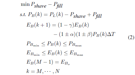
This subsection describes the fundamental peak shaving formulation. This algorithm is used to determine the charging and discharging schedule using the load data.

where
3. Wind Power Generation Forecasting Based on Fuzzy Modeling
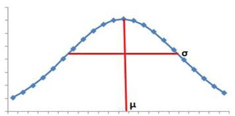
In probability theory, a normal or Gaussian distribution is a very commonly occurring continuous probability distribution. Normal distributions are extremely important in statistics and are often used in the natural and social sciences for real-valued random variables whose distributions are unknown.
Different probability distribution functions may be selected for different kinds of uncertain values [10]. The normal distribution function is used in this paper. The general formula of the probability density function for a normal distribution with uncertain variable x is given below:

where
Power load data, especially for residential loads, are variable and uncertain. For example, the variability of the electricity consumption of a single residential customer generally depends on whether family members are home and on the time of use of a few high-power appliances with relatively short usage durations during the day, and is subject to very high uncertainty. Probabilistic analysis and fuzzy theory can be used to analyze the uncertainty of the load [11].
A method for describing a membership function involves the application of data on the average value m and maximum error e of the input quantity. In practical applications, this method may be used to describe the values of wind power generation. In this case, the fuzzy parameters can be defined as follows [12]:

where e is the maximum error.
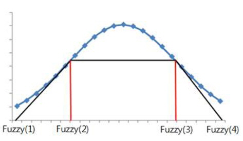
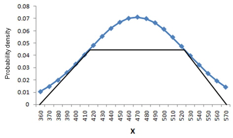
A trapezoidal fuzzy curve can be drawn using Eq. (4) and is shown in Figure 2. This paper calculates the fuzzy percentage using this curve. Four fuzzy forecasting wind power generation curves are made using these percentages. The formula for calculating the percentage is as follows:

Wind power generation data are forecast using these four fuzzy forecasting wind power generation curves for real-time peak shaving. If the real wind power generation at an arbitrary point is smaller than the value of
In the real-time operation, the applied level of wind generation is based on the fuzzy wind model at the following time period, which depends on the wind generation level at the previous long-term time unit. When the error between the real and forecast wind generation values is less than
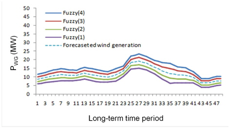
This section describes the process of creating the trapezoidal fuzzy curve and gives corresponding examples of the application of the peak shaving algorithm. The wind power generation was classified on an hourly basis to generate the trapezoidal fuzzy curve and each fuzzy percentage. Thereafter, a normal distribution was made using the wind power generation data with respect to time. Figure 3 shows a trapezoidal fuzzy curve that was drawn using this method. The fuzzy model might have different values over the entire period. This paper uses a 48 × 4 matrix that includes the end-points of the trapezoidal models at all the periods using historical power generation data with 30-min intervals. Table 1 lists the percentages of the endpoints of the fuzzy model at each time period in reference to the expectation, as determined in this paper.
[Table 1.] Percentages of end-points of fuzzy model for wind power generation
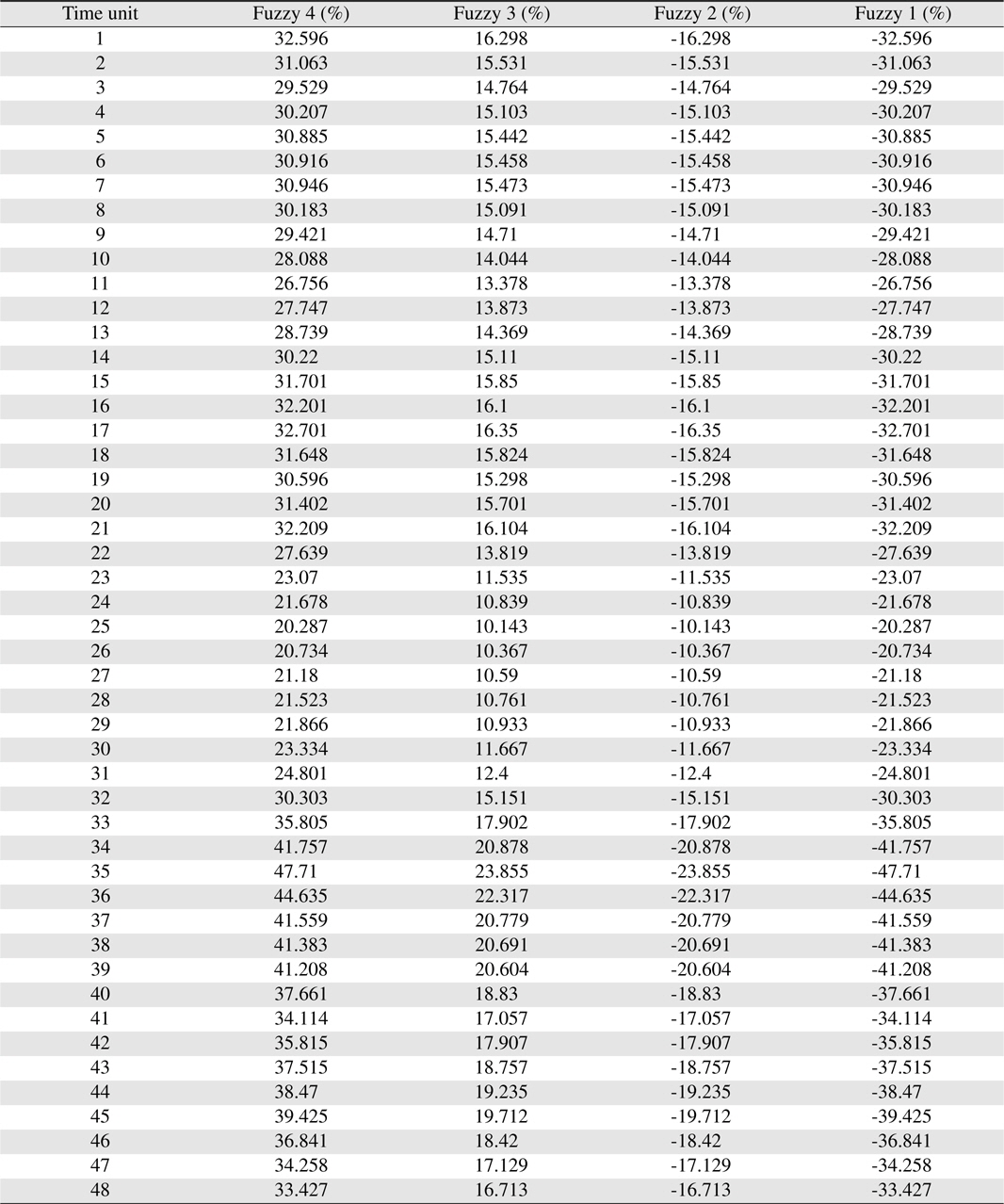
Percentages of end-points of fuzzy model for wind power generation
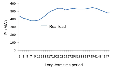
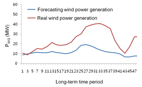
The same fuzzy model could also be applied to load curves, as in [7]. However, in [7], the method used for the fuzzy model construction was not mentioned. This paper adds wind power generation data to the grid and performs real-time peak shaving under the assumption that the real load data are obtained. This paper illustrates the applicability of a fuzzy curve for wind power generation data. Figures 4 and 5 show the real load curve and real wind power generation curve, respectively. Figure 6 shows four fuzzy curves based on the forecast wind power generation curve. In Figures 4–6, the x-axis denotes the longterm time unit (30 min) intervals over the course of a day.
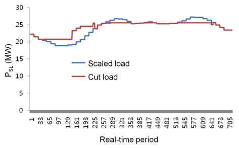
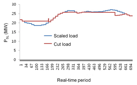
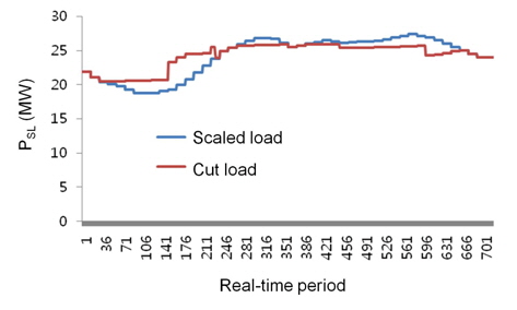
Figure 7 shows the peak shaving results using real load and real wind power generation data. Figure 8 illustrates the peak shaving results using real load and forecast wind power generation data. Figure 9 shows the peak shaving results using real load and wind power generation data after the application of the fuzzy model. In Figures 7–9, the
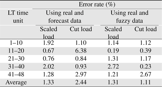
In a real-time simulation performed using the developed realtime mode emulator, one day is divided into five portions, and each portion starts from an long-term time unit: 1, 11, 21, 31, or 41. This is because different errors are expected between the real and forecast values of the wind power generation data at each portion. In other words, the error rate might be different depending on the time of day. Table 2 lists the error at each longterm section, 1–10, 11–20, 21–30, 31–40, and 41–48, compared to the results when using the real wind power generation data. In the process of peak shaving, the effective load was adopted, which is the load subtracted by the wind power generation. As listed in the table, the error rates at each section are smaller when using the fuzzy model of wind power generation. The same characteristic is seen in the overall error rate.
[Table 2.] Error rate of peak shaving results

Error rate of peak shaving results
This paper presented long-term cycle control strategies for a large-scale BESS. The main focus of this paper was illustrating the applicability of a fuzzy model for the forecast wind power generation as an input for real-time peak shaving. This operation mode could be used to perform an energy time shift, and minimize the threshold value obtained from the difference between the upper and lower loads. This paper included an illustrative example showing the performance of the algorithm with real load and wind power generation data using real, forecast, and fuzzy model-based curves with the developed real-time operation simulator.