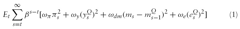
Over the years, many countries around the globe have adopted monetary targeting (MT) regimes under different circumstances. This has been the case of many advanced economies, in which this strategy has been in place for a prolonged period of time in the postwar era.1It is sometimes claimed that the Bundesbank’s and the Swiss National Bank’s outstanding record of inflation control stemmed fromtheir use of monetary targeting.The extent towhich these central banks have actually adhered to the strict anti-inflationary form of aMT rule, or instead have adopted a more pragmatic approach, has been a matter of debate. A number of economies belonging to the sometimes called ‘US dollar bloc’, such as Australia, Canada, and New Zealand (Collins&Siklos, 2004), have also implemented MT strategies in the past. The decision of these economies to switch to inflation targeting from the very end of the 1980s onwards is related to the difficulties with using MT under conditions of financial innovation that led to instability in the velocity of money.2 It is worth mentioning that, while not following a MT approach, the Eurosystem has adopted a monetary policy framework that emphasises the role of monetary aggregates (see European Central Bank, 1999).
Among emerging market economies (EME), a rich variety of experiences provide us with evidence of the widespread use of MT over time. Currently, the world’s largest EME, China, follows a monetary strategy that is best characterised as MT (Koivu
Considerable research has been devoted to uncovering central bank preferences. The empirical literature on optimal monetary policy has largely focused on the US, which is not anMT(nor an IT) country. Related work for other countries has focused on IT experiences, such as other advanced economies (Collins & Siklos, 2004) and the EME case of South Korea (Sánchez, 2009). Our paper extends the literature providing first estimates for an MT central bank’s objective function – namely, the National Bank of Romania’s (NBR) in the period 1999–2005.4 Our evidence on NBR’s policy intentions at that time is also meant to be a useful point of reference for the analysis of Romania’s ongoing IT regime (announced in August 2005). In this regard, the transition to IT has been smooth and decided well in advance by the NBR authorities, with a rigorous assessment of current policy intentions being out of the question due to the short period elapsed since the launch of IT – a period in which the country was also subjected to significant external shocks. While no estimates of central bank preferences are to date available for Romania, European Institute of Romania (2004) characterises NBR reactions in terms of borrowed reserves responses to inflation and the value of the leu. Estimated responses are appealing since they capture the systematic relationship between the monetary policy instrument and macroeconomic variables and, as such, they can be viewed as approximations to central bank decision rules. The main limitation of estimated policy rules is that they are unable to address questions about the policy formulation process, as they fail to uncover central bank preferences. The identification of optimal policy weights attempted here offers the advantage of unveiling the monetary authority’s objectives.
Our study addresses two questions concerning the operation of anti-inflationary monetary policies, namely, general issues (in particular, instrument smoothing) and the more specific aspects relating to Romania’s EME status. With regard to the former, our assessment of Romanian policy in terms of instrument smoothing is relevant given the experience of countries explicitly targeting inflation, with smoothing in the present case referring to base money growth instead of the interest rate. With regard to the latter instrument, smoothing has been documented for advanced economies (Collins & Siklos, 2004; Dennis, 2006; Ozlale, 2003) and South Korea (Sánchez, 2009). Moreover, we evaluate in a Romanian context the question of whether monetary policy was concerned about exchange rate stability – an issue particularly relevant for emerging market economies (EME). According to Calvo and Reinhart (2002), EMEs have special characteristics that would motivate their ‘fear of floating’, i.e. their desire for a relatively small degree of exchange-rate flexibility. One possible explanation for this is that a devaluation/depreciation would induce unfavourable balance sheet effects by increasing the domestic-currency real value of external liabilities, thus provoking a drop in economic activity (the so called ‘contractionary devaluations’).5 It is worth saying that, even if the evolution of the exchange rate does not constitute a direct concern for monetary policy, it may still matter indirectly through its effect on other potential policy goals such as inflation. Although the NBR had price stability as it main policy goal and the leu was officially floating, it has been pointed out (e.g. OECD, 2002) that Romania pursued an implicit exchange rate crawling peg during the MT period. This notion of a (successful) de facto peg is however not substantiated by the data (Firdmuc and Horváth, 2008; Frömmel & Schobert, 2006). To have a more clear idea about the facts, we complement our estimation of policy weights with the analysis of key macroeconomic indicators during the MT period, as well as in the periods immediately before and after that.
We look at the conduct of monetary policy in Romania over the period 1999–2005. The reason why we begin our analysis in 1999 is that, in the two years before that (which can also be classified as MT), Romania was affected by considerable macroeconomic instability as the country adjusted to the launch of an IMF-supported programme and faced unfavourable international conditions. In order to examine the relative short period 1999–2005, we resort to monthly data, employing smoothed versions (more concretely, rolling quarterly moving averages) for candidate monetary policy objectives that could be affected by high-frequency volatility.
Technically speaking, Ozlale’s (2003) US study comes closest to ours. This author employs maximum-likelihood methods to uncover central bank preferences conditional on private sector behaviour. Dennis (2006) proposed a different methodology, jointly estimating the macro-model and monetary policy weights. Otherwise, the latter study, like Ozlale (2003), employs Rudebusch and Svensson’s (1999) model to describe the macroeconomy and uses an infinite horizon quadratic objective function.6 One caveat with this literature – one that also applies to the present study – concerns the absence of forward-looking elements in the empirical macro-model. In acknowledgement of this limitation, we adopt a seemingly unrelated regression approach to estimation of the macromodel – a technique allowing for correlation across simultaneous equation errors. Another way in which we depart from the studies mentioned in this paragraph relates to the introduction of the money market equilibrium and small-openeconomy features.Drawing on Collins and Siklos’ (2004) and especially Sánchez’s (2009) studies for other small open economies, these features involve – in addition to the NBR’s concern for exchange rate stability – the role of the exchange rate and external variables in affecting the Romanian macroeconomic developments.
The structure of the paper is as follows. Section 2 outlines the main characteristics of Romania’sMT regime, also comparing key macroeconomic developments at the time with the periods immediately before and after it. Section 3 describes the paper’s theoretical approach and empirical methodology. Results and policy implications are discussed in section 4. Section 5 offers concluding remarks.
1See, for example, Gerlach & Svensson (2003), Laubach & Posen (1997) and Mishkin (2001). 2See, for example, the description in Guttmann (2005) for the Australian case. 3Price stability has instead been made the primary objective of Korea’s inflation targeting regime since 1999 (Sánchez, 2009). 4The loss function parameters indicate how different goals are traded off in response to shocks. They are estimated under the assumption that the NBR sets monetary policy optimally, conditional on economic outcomes and an empirical macro-model. 5A weaker currency is generally found to be contractionary in the empirical literature, even after including a number of different controls. Concerning liability dollarisation, see for example Céspedes et al. (2004). Those discussing the implications of contractionary depreciations for monetary policy include Eichengreen (2005), and Sánchez (2007, 2008). 6Technically, we are not influenced by other attempts at characterising monetary policy intentions, such as Favero and Rovelli (2003) and especially Cecchetti and Ehrmann (2002).
2. Monetary Targeting in Romania
This section describes the main aspects of MT in Romania over the period 1999–2005. Already at that time, the NBR had the main objective of ensuring and maintaining price stability. Without prejudice to this primary goal, it was envisaged that theNBRwould support ‘general economic policy’, i.e. aim at preserving economic stability more broadly defined. Romania had been pursuing policies related to MT from the first half of the 1990s. During the first years of the transition period (from 1991 to the first half of 1993), the NBR attempted to directly control a broad monetary aggregate (M2). From the second half of 1993, after having created the basis for exerting indirect control over the money supply, the central bank turned to base money (M0, i.e. currency in circulation plus deposits with the central bank) as an operational objective of monetary policy (Gherghinescu & Gherghinescu, 2008). The period until 1996 was marked by the pre-eminence of exchange rate stabilisation over MT considerations. This, together with unstable macroeconomic conditions in the period 1997–1998,7 prompts us to delay our starting date to 1999. During the period of interest, NBR’sMT strategy used M0 as the operational objective and M2 as the intermediate objective. Popa
In terms of communication strategy, during the MT era, NBR annually submitted to Parliament a report on the monetary policy conducted in the previous year and the guidelines for the current year, being accountable for attaining its objectives.TheNBRreleased monthly bulletins, annual reports and press releases, whereby it explained to the general public its views about developments in real economy and financial markets, as well as concerning monetary and foreign exchange policy decisions. The central bank also informed, through this channel, the reasons why the inflation objective was not met. The NBR also engaged in communication with the public via various presentations and speeches by top officials. With regard to relevant requirements for EU membership, over the period of interest, the Romanian government submitted its Pre-Accession Economic Programmes, including a number of aspects relating to monetary policy, such as central bank independence (Dvorsky, 2004, 2007).
From the point of view of policy management, Romanian authorities had to cope with some structural characteristics affecting the market for money. The existence of a large informal sector in Romania created some complications as the sector’s demand for cash (both domestic and hard currency) was rather difficult to predict. Another challenging factor was the large degree of dollarisation/euroisation in the economy. In addition to a large fraction of money supply being in euros and US dollars, indexation of financial contracts in foreign currency was widespread. Dollarisation/euroisation contributed to hampering the implementation of monetary policy by constraining the central bank’s control over money supply (Daianu & Lungu, 2007).
The NBR announced its official adoption of the IT regime in August 2005. The NBR explained the latter policy move as a response to the increasing inadequacy of monetary targeting approaches (NBR, 2005). Inflation targets had been made public prior to the switch to IT. For instance, the end-2005 inflation target was initially set at 7%, then changed to a target band of +/− 1% centred on 7.5%, which compares with actual inflation of 8.6% – slightly above the upper band.
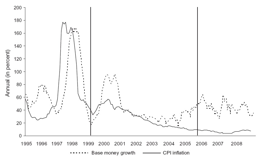
The MT strategy carried out by the NBR over 1999–2005 led to a gradual disinflation process (see Figure 1).9 For most of this period, disinflation proceeded alongside a decrease in (nominal) base money growth. However, starting in the second half of 2004, disinflation coexisted with increased base money growth, which points to an ongoing strong monetisation process. Table 1 allows us to look in more detail at macroeconomic developments (including those in inflation and monetary trends), distinguishing between the period of the first half of the 2000s – roughly covering the MT period under study – and two proximate periods before (1995–1998) and after that (the initial years of IT since 2006).10 As mentioned earlier, Romania’s experience in the second half of the 1990swas surrounded with significant macroeconomic and financial instability (Budina
With regard to consumer price developments, the period 1995–1998 preceding the MT period under study was characterised by high rates as well as large swings in headline inflation (Figure 1 and Table 1). Not only the level but also the variability of inflation dropped considerably over the MT period. This process appeared to continue since the launch of IT – a development that can be confirmed by looking at core inflation measures – even if the gains have not been very large compared with the end of theMTera. This should, however, be seen against the background of sizeable external shocks facing the Romanian economy over the last few years – an aspect we turn to later in the present section. Moreover, it must be borne in mind that any analysis of the IT regime has to be interpreted very carefully in light of the short time span elapsed since its implementation. Monetary trends largely mirrored what was said about inflation volatility for the MT period, with the variability in base money growth declining at that time. While remaining at a much lower level than in the second half of the 1990s, base money growth volatility increased somewhat in the IT regime, possibly reflecting the change in the instrument of monetary policy to the interest rate or the nature of the intensified monetisation process seen since about the mid-2000s. In the MT period, the autoregressive component of nominal base money growth declined, but that of this variable in real terms increased slightly. In the context of the policymaker’s optimisation process (conditional on an empirical macro-model), we shall later empirically assess whether base money growth smoothing was a significant motive on the part of the NBR. Turning to nominal (money market) interest rates, they exhibited a downward trend and became more predictable over the years.
[Table 1.] Summary statistics: 1995Q1?2008Q2
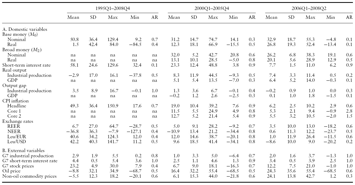
Summary statistics: 1995Q1?2008Q2
Concerning the real economy, real output growth improved considerably in the MT period, judging from a brisk industrial production expansion that contrasted with the drop registered in the period 1995–1998. While decelerating slightly over the IT period, industrial production growth became at the time even more stable than in the MT era. The more broad-based information conveyed by real GDP growth instead points to a faster pace of expansion and marginally lower variability since 2006. Output gap volatility (based on industrial production data) appears to have decreased markedly in the MT period, a process that continued into the IT period; the latter continued decrease is only marginally detectable in the case of real GDP data.
Exchange rate fluctuations turned much smoother in the MT period, judging from the summary measure given by NEER’s standard deviation as well as the corresponding statistics for bilateral exchange rates. Having said this, the degree of exchange rate volatility remained considerable in the first half of the 2000s, and in particularmuch higher than the same measures computed by Sánchez (2009) for South Korea in its IT period, 2000–2006 – another experience of officially floating exchange rates. While the nominal exchange rate of the leu depreciated over the entire decade 1995–2005, the secular trend appeared to be one of REER appreciation, which even extended into the IT era. One factor behind this is sizeable capital inflows into the country. The considerable flexibility of the leu witnessed ever since the MT regime has occurred despite foreign exchange intervention underpinning Romania’s fast-expanding international reserves.
Let us finish by discussing the evidence on whether the decline in macroeconomic volatility in the MT period can be attributed to the higher predictability of external variables. This is not found to be the case for the G7 variables considered (industrial production, interest rates and stock prices) whose variability increased from the period 1995–1998. Neither does this notion receive support from the fluctuations in oil and non-oil commodity prices, which – mostly due to the latter group – became on balance wider. In addition, during the MT era, the Romanian economy was hit by considerable rises in both categories of prices, in contrast with the drops observed in 1995–1998. In comparison with the first half of the 2000s, the IT period benefited from some reduction in the volatility of G7 variables, but had to withstand similarly high variability, as well as even stronger rises, in oil and non-oil commodity prices.
In sum, the evidence presented here points to an improved macroeconomic performance in Romania in theMTperiod compared with the period 1995–1998. In this regard,we find evidence that the level and volatility in inflationwent down, and so did output gap variability. Moreover, we observe smoother fluctuations in base money growth – the policy instrument under the MT regime – as well as in interest rates and exchange rates. However, exchange rate variability remained considerable under the MT scheme, which suggests the lack of a ‘fear of floating’ motive behind NBR policy moves. The less predictable developments in external variables such as G7 macroeconomic aggregates and world commodity prices witnessed during the MT scheme suggests that the improvement in Romanian macroeconomic performance during the first half of the 2000s may not stem from ‘good luck’ (as given by international developments outside the authorities’ control).
7These conditionswere given by drastic macroeconomic adjustment in the context of an IMF-backed stabilisation programme and an adverse international environment (Gabor, 2008). 8The growth rate of Romanian foreign reserves induced by capital flows remained high at the start of the IT regime. This is partly due to substantial liberalisation of the capital account in early 2005 and anticipations of EU accession in 2007. 9See section 4 for a description of the main data series used in Figure 1 and Table 1. Additionally, BIS data are employed for core inflation measures, real GDP and bilateral exchange rates. Two core inflation measures are used: core 1 excluding volatile (vegetables, fruit, eggs, fuel) and administered prices, and core 2 excluding only administered prices. The external variables included in Table 1 are a subset of all those considered in our analysis. 10The reason for dropping year 1999 from this period is that we lack quarterly data for some variables (M2, core inflation measures and real GDP). The results reported here for other variables would be substantially unchanged if we included year 1999.
This section focuses on the central bank’s optimisation problem, conditional on a macro-model describing the rest of the economy. We adopt a Rudebusch and Svensson (1999) setup, extended to accommodate for money balances and open-economy features.The latter include: (a) modelling the exchange rate and its implications for inflation and output fluctuations; and (b) controlling for external variables that influence Romania’s macroeconomic developments. We postulate that the monetary authority’s instrument is

where

is three-month moving average of the output gap

is the three-month moving average of the REER(in deviation from its trend) and

is the three-month moving average of
The rest of the economy is determined by the following equations:


where
The market for money deserves further discussion. Our money demand specification allows not only for standard determinants (income and interest rates), but also for the exchange rate. In this regard, Romania is a small open economy where international trade liberalisation during the transition process arguably affected money holding behaviour, allowing agents to more easily switch between foreign and domestic currencies. In the literature on money demand for new EU Member States (NMS), analysts (Buch, 2001; Orlowski, 2004) have included as a regressor the exchange rate against the euro. However, the euro was only introduced in January 1999 (and in circulation only in January 2002). Prior to that, for many NMS either the US dollar or the German mark has been the most important currency (Beguna
The macro-model is estimated using a seemingly unrelated regression (SUR) methodology.We favour SUR over OLS because the former enables the error terms to be correlated across equations, in acknowledgement that our model is too simple to be deemed fully structural. Moreover, it is worth saying that, according to statistical significance, the estimated version of the model may fail to include some of the terms generally allowed for in equations (2)–(5).We employ monthly data ranging from 1999:1 to 2005:12.13 The series for the short-term (threemonth) interest rate – theROBID (Romanian Interbank BidRate) – and monetary aggregates are obtained from the NBR. The data on real output (measured as an industrial production index) and headline CPI are from the International Monetary Fund’s International Financial Statistics (henceforth IFS). REER and NEER data are from IFS and BIS, respectively (an increase being defined to mean an appreciation). Concerning global variables in
The central bank’s problem is to minimise (1) subject to equations (2)–(5). The solution yields the central bank’s optimal reaction function. Because the loss function is quadratic, the optimal reaction function is linear in the forcing variables:

where
[Table 2.] Weights used in central bank loss function
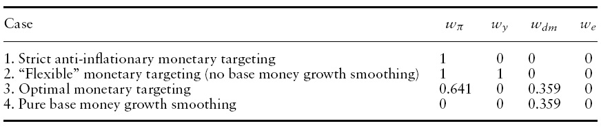
Weights used in central bank loss function
In order to better understand NBR intentions we consider two types of loss functions (Table 2). First, we consider two rule-of-thumb benchmarks: (a) strict anti-inflationaryMT, namely a central bank that focuses exclusively on inflation; and (b) ‘flexible’MT, which assumes that the NBR cares about both inflation and output (
11More specifically, we define variable where z = m;y;e. Notice that this averaging simply amounts to attaching weights in the loss function to objective variables over more than one period.This does not affect the time series properties of the errors in the macromodel equations (2) through (5) below. The estimation of these equations employs no moving averages of the data. 12Note thatwe allowfor contemporaneous effects of the nominal interest rate and NEER on money demand. The model is closed with a PPP constraint: . 13The Appendix contains the details of our estimation. Estimating the model until the announcement of the IT regime (August 2005) did not substantially change any of the results reported below. 14Our use of a two-step method (first estimating the macro-model, then, conditional upon the latter, obtaining the policy coefficients) allows us to consistently compare the optimal central bank’s loss function with rule-of-thumb benchmarks for the policy weights, conditional on the same empirical macro-model. 15Which specific type of normalisation we adopt is inconsequential. The only thing that matters for representing central bank preferences are the relative weights between all possible objectives.
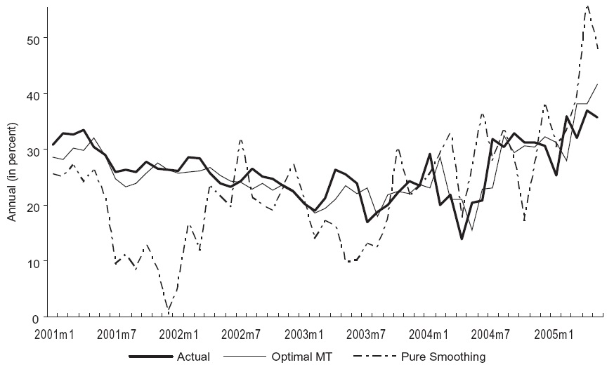
The methodology used here identifies optimal policy on the basis of an empirical macro-model and a postulated infinite horizon loss function for the policymaker. This section presents the model results in terms of a comparison between actual base money growth rates and paths obtained by simulating the optimal reaction functions (conditional on the set of policy weights that we employ). More specifically, we compare actual base money growth rates (thick lines in all Figures 2 through 4) with the scenarios described in section 3, which consist of a number of rule-of-thumb benchmarks and optimisation-based paths (Table 2). We also report correlation coefficients between simulated and actual base money growth rates (see Table 3).
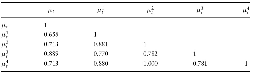
Underlying all base money growth paths are the set of weights reported in Table 2. Concerning theweights that are based on optimisation and thus estimated (lines 3 and 4 in Table 2), the empirical results involved are reported in Table 4. The estimate for
[Table 3.] Correlation matrix for different base money growth paths

Correlation matrix for different base money growth paths
We thus find that the NBR attached a negligible emphasis on both output and the exchange rate. The latter two variables however play indirect roles in the determination of inflation, and thus of monetary policy itself. Inspection of our estimated macro-model allows us to see that inflation is directly affected by REER (see equation (A.2) in theAppendix). Output influences inflation indirectly, given that it enters money demand function (A.4), thus affecting interest rates and – indirectly via equation (A.3) – the exchange rate, which in turn impacts inflation, as we have just seen.16 In sum, even if they are not monetary policy objectives, output and exchange rates indicators are worth being monitored on a regular basis by the NBR.
[Table 4.] Estimates of central bank objective function parameters
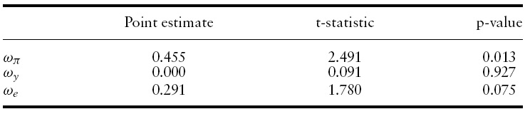
Estimates of central bank objective function parameters
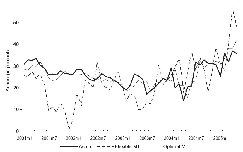
Figures 2 and 3 contrast the rates of base money growth that a strict antiinflationary and flexible monetary targeter, respectively,would have selected (each one depicted as dashed lines) alongside the corresponding actual rates.17 The Figures indicate that Romania did not pursue strict anti-inflationary nor flexible MT. Under the latter two regimes, base money growth rates would have varied much more than observed in reality. A better approximation to reality is given by optimal MT – its associated path being represented (as a thin solid line) in both Figures 2 and 3. This finding is consistent with the higher correlation with actual base money growth shown by the implied optimal MT path in comparison with strict anti-inflationary and flexibleMTpolicies – a superiority that also extends to the case of pure instrument smoothing discussed in the next paragraph (Table 3).
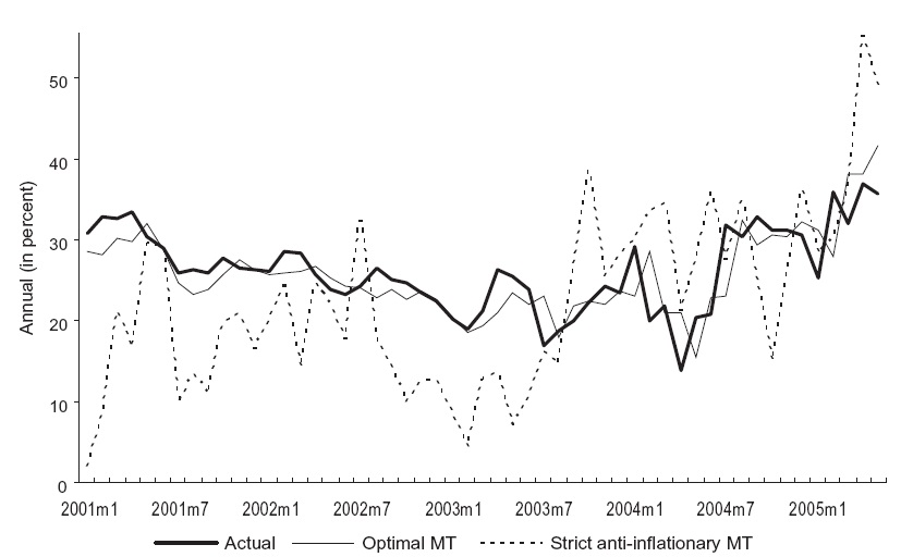
In Figure 4, we report actual money growth rates alongside optimalMT(again as a thin solid line) and another optimisation-based path, namely, that resulting from constraining the inflation policy weight to zero (i.e.
[Table 5.] Encompassing tests for simulated base money growth paths
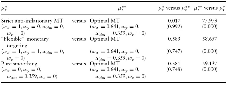
Encompassing tests for simulated base money growth paths
Visual inspection of the alternative base money growth paths is informative, but a more formal exercise can be conducted by comparing them using the encompassing test (Hendry, 1995; see the application in Collins & Siklos, 2004). The latter tests allow us to check for the statistical significance of the base money growth paths suggested by candidate reaction functions against each other. The aim is to determine whether one reaction function statistically dominates a given alternative by better tracking actual base money growth rates.The test is based on regressions of the form
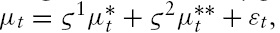
where

and

are the corresponding rates as implied by any two competing reaction functions. We discriminate between one of these two competitors using Wald tests of the form: H∗ :

would be said to encompass

(and vice versa).
Table 5 shows the results of our encompassing tests. All tests corroborate what stems from visual inspection of Figures 2 through 4. The optimal base money growth path appears to encompass all of its three alternatives at the 5% significance level. In contrast, neither of these alternative paths – namely, strict anti-inflationaryMT, flexibleMTand pure instrument smoothing – encompasses the optimal base money growth path.
Summarising this section thus far, our characterisation of the MT regime in Romania reveals that monetary policy evinces a dominant concern for price stability, while also displaying a considerable role for instrument (that is, base money growth) smoothing. Given these two objectives, increasing the weight that the National Bank of Romania (NBR) places on potential additional goals (such as the variability in output gaps and exchange rates) appears to be redundant, not helping simulated optimal base money growth rates track the policy decisions significantly more closely. Finally, optimal policy thus characterised is shown to better track base money growth paths than the two benchmarks considered, namely, strict anti-inflationary and flexible MT.
Although the literature usually reports that interest rate smoothing is an important characteristic of central banks, a consensus has not yet been attained regarding the link between instrument smoothing and concerns about output variability. Monetary policy inertia is often associated with the idea that wide fluctuations in interest rates may imply a reputation or credibility loss if the policy decision is reversed in the near future. Policymakerswould also tend to be cautious when changing interest rates due to parameter uncertainty (Sack, 2000). Yet other reasons for smoothing conveyed in the literature involve forward-looking expectations (Woodford, 2003) and data uncertainty (Orphanides, 2003). All these approximations to smoothing rely on the absence of any connection between instrument smoothing and output stability concerns. Adopting this perspective and applying it to an MT context, Romania would have engaged in a gradualist approach to inflation fighting coupled with a neglect for output variability. This would be broadly consistent with the NBR’s mandate, which has price stability as its main goal. An alternative interpretation of the nexus between interest rate and output stability is advanced by Collins and Siklos (2004). According to these authors, considerable interest rate smoothing could be seen as indirect evidence of concerns for output variability. This view is based on Svensson’s (1999) notion that IT central banks adopt a policy imbued with a sense of gradualism or flexibility under three circumstances: emphasis on output stability, model uncertainty and interest rate smoothing. In particular, monetary authorities could engineer smooth changes in interest rates so as to stabilise economic activity. Applying this logic to Romania, despite our failure to identify a positive weight on output, the NBR could be seen as indirectly concerned for output variability in light of strong base money growth smoothing. The notion that the NBR followed a gradualist approach toward inflation and output stabilisation would be roughly in line with Romania’s monetary policy framework – which envisages a secondary role for economic stability. In sum, the two interpretations given here for the link between instrument smoothing and output stabilisation are broadly plausible characterisations of Romania’s MT scheme. It is however worth noting that these two views convey different implications for the role that output stability played in NBR policy moves.
Finally, let us further discuss our finding that theRomanian monetary authority does not appear to be concerned about exchange rate movements. This result is still compatible with the idea that the NBR looks at realisations of the exchange rate as a leading indicator for inflation developments. Furthermore, the lack of an explicit concern for exchange rate variability is in line with the evidence about the leu’s considerable flexibility during theMTperiod.Romania has intervened in the foreign exchange market over theMTperiod, but without preventing the value of the leu from fluctuating considerably. As therewere at that time signs of decreased inflation, output and interest rate variability compared with the immediate past, we cannot conclude that such interventions were in conflict with NBR’s pursuit of price stability.18
16The demand for output reacts (negatively) to the exchange rate (see equation (A.1) in the Appendix). This can be rationalised in terms of the adverse effect of the exchange rate on competitiveness. 17More specifically, actual base money growth rates depicted in Figures 2 through 4 correspond to smoothed (six-month moving averages) transformations of annual growth rates. Simulated paths are not smoothed, as they are already derived from an optimisation involving smoothed goals. 18This analysis concerns Romania’s actual experience with MT. Sterilisation of capital flows did not become a destabilising force before the regime’s replacement by IT.
Romania’s experience withMTin the period 1999–2005was broadly satisfactory, in particular contributing to reducing inflation from very high and unstable levels. While not interfering with the aim of bringing inflation rates down over time, the technical problems known to be involved in applying monetary targeting (e.g. conjunctural instability of money demand, ongoing financial innovation) may have limited the effectiveness of MT. We find that Romania’s MT regime can be characterised by concerns for both price stability and base money growth smoothing. Exchange rate variability and output stability are instead found to be redundant. These results deserve further discussion, to which we devote the remainder of this section.
Our results shed some light on both general issues concerning monetary policy (in particular, instrument smoothing) and the more specific aspects relating to Romania’s emerging market status. With regard to the former set of issues, our characterisation of Romanian policy in terms of instrument smoothing is in line with the experience of countries explicitly targeting inflation, although smoothing in the present case is related to base money growth instead of the interest rate. In line with the inflation targeting literature, we have provided two different explanations for our results. First, base money growth smoothing can be seen as independent from NBR concerns for output stability. Adopting this standpoint, our findings should be interpreted as capturing a gradualist approach to disinflation, coupled with a neglect for output variability. This is consistent with Romania’s MT framework, which had price stability as the primary monetary policy objective. Second, our results can be rationalised in a second way, along the lines of Collins and Siklos (2004). These authors draw on Svensson (1999) and, keeping within the boundary of IT, interpret the result that central banks evince strong interest rate smoothing as indirectly reflecting some concern for output stability. In analogy to this, the NBR could be seen as adopting a flexible policy in which monetary policy inertia (concerning base money growth) aims at mitigating output volatility. This is broadly in line with NBR’s acknowledgement of a (secondary) output stabilisation goal. All in all, both interpretations of smoothing presented above can be deemed broadly compatible with NBR’s mandate, although they imply contrasting views concerning how crucial output variability was for Romanian monetary authorities under the MT regime.
In connection with Romania’s status as both a very open economy and an EME country,we assess the role of exchange rate variability in monetary policymaking. The result that the exchange rate does not appear to be a direct monetary policy concern resembles Sánchez’s (2009) finding for inflation targeting in South Korea. This result is consistent with considerable exchange rate flexibility during theMT regime, despite moderation from the high instability seen in the second half of the 1990s.While Romania intervened in the foreign exchange market to stem pressure from capital inflows at some points during the MT period, the value of the leu has fluctuated over time, with fewer signs of variability in inflation, output gap or interest rates than prior to MT. Finally, the lack of direct concern for exchange rate variability did not prevent the NBR from responding to movements in the value of the leu given their possible impact on inflation.
As in customary in studies of transition and emerging economies, our results for Romania should be interpreted carefully, for instance in light of the structural transformations that accompanied the macroeconomic processes under investigation and the relatively short period over which the monetary targeting regime was in place.