Orbit determination methodologies were originally proposed by Gauss and Laplace to solve orbit determination problems for celestial bodies such as planets and minor planets (Schaeperkoetter 2011). The demand for orbit determination rose with the 1801 discovery of the minor planet Ceres, and orbit determination technology was needed to find the minor planet passing the Sun. Gauss succeeded in re-finding the position of the Ceres in December 1801 using the Gauss method, which is an effective method of orbit determination based on planetary observation data. The Laplace method is based on three observation values, and with the second value as a reference, two nearby observation values are used for orbit determination. As the space race was incepted, the Laplace method was proved to be ineffective with the low Earth orbit objects. This method has been usually applied to heliocentric orbits. Later, in 1889, Gibbs modified the Gauss method with his own technique. This orbit determination method was utilized for orbits in deep space, rather than near space.
In Korea, various studies exists on orbit determination for artificial satellites. Kim et al. (1987) examined numerous orbit determination methods, focusing on preliminary orbit determination and orbit derivation from differential correction. Lee et al. (2004) utilized actual optical observation data in their study, using both the preliminary orbit determination process and simulation results for the precision orbit determination of low orbit satellites. For precision orbit determination, Lee et al. (2004) concluded that there should be at least two optical observation systems, multiple observatories in operation, and an adequately sufficient amount of observation data. Choi et al. (2009) stated that precise optical observation can be obtained using a narrow viewing angle telescope, a CCD with small pixels, and an SLR. While Korea domestically has seen various theoretical and practical studies on orbit determination since 1986, few studies exist that consider on-site operations. Currently, most ground operation center performs the Geosynchronous Earth Orbit (GEO) satellite orbit estimation independently with the ranging and angle measurement in Korea (Lee et al. 2011; Lee et al 2012). Korea does not have any dedicated optical satellite observation system yet. However, we can observe space objects optically and estimate their orbit in our visible region with an optical observation system as they reflect Sun light with proper relative position.
In this study, we examined the effects of baseline distance variation between optical observatories on orbit estimation precision with optical observation of artificial satellites. Observation data was simulated, and orbit determination was performed using data obtained from multiple optical observatories. The study attempted to present results that would be valuable for site selection for artificial satellite optical observatories in the future. Since the Korean peninsula has a latitudinal axis that is much longer than the longitudinal axis, possible positions were classified according to latitude. The difference in baseline distance between the observatories was assumed to be 50 km each, and comparisons were made using simulations performed at each site. Since this study relies on simulations, white noise was introduced to reflect more realistic conditions in the generated observation data.
The following sections describe the characteristics of geostationary satellites and orbits, and explain the conditions for optical observations through telescopes and backend sensors. Lastly, this paper explains the characteristics of the Orbit Determination Tool Kit (ODTK) orbit determination program used in the initial orbit determination of geostationary satellites, and analyzes simulation results.
2. OPTICAL OBSERVATION OF GEO SATELLITE
2.1 GEO Satellite and Orbit Characteristics
The COMS satellite targeted in this study is a multipurpose satellite in geosynchronous orbit. Geostationary orbit is 0° of inclination among geosynchronous orbit. The concept of geosynchronous orbit was first proposed by Constantin Tsiolkovsky in the 1920s, but became widely known after Arthur C. Clarke published a 1945 article on the adequacy of geosynchronous orbit for communications satellites (Clarke 1945). Geostationary satellites are located above the equator at an altitude of 35,786 km and have an orbital period of one sidereal day, thus maintaining the same sub-satellite point (Kelecy et al. 2008; Kelecy & Jah 2011). The fixed position of artificial satellites from the Earth surface allows continuous observations of such satellites.
Due to the characteristics of an optical observation, we have two restrictions from the terrain topography of the observatory and from the relative positions of the Sun from the space objects (Birney et al. 2006). To minimize the restrictions for the terrain environment and low altitude passing of a satellite, the location of an observatory usually is chosen near the top of the mountain with open field of view. As a GEO satellite is located at 35,786 km above the Earth’s surface, we can observe the orbit with the proper relative position of the Sun (Lowe et al. 2010). First, Sun must set enough under the horizon of an observatory to have fairly dark sky for the detection of the satellite. Second, Sun must be at the proper relative angle from the satellite to reflect enough Sun-light except the eclipse in the Earth’s shadow.
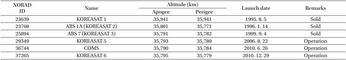
[Table 1.] GEO satellite list in Korea (Jan 2015).

GEO satellite list in Korea (Jan 2015).
As of January 2015, Korea has launched six geostationary satellites, and three are still in operation.
2.2 Characteristics of Optical Satellite Observation
While Lippershey is known as the inventor of the telescope, it was Galilei who first made observations of celestial bodies. However, the telescope used by Galilei was inappropriate for Astronomy as it had a narrow angle and low magnifying power. Keppler developed a refracting telescope but the lens caused chromatic aberration with the dispersion of light. Newton resolved this problem by developing a reflective telescope, which can be classified into various types depending on the method of gathering and expanding light. Clear observations can be made since there is no chromatic aberration (Kim et al. 2006).
Among the many developments of optical telescope systems, the most prominent involved the backend sensor, which were traditionally used in cameras and camcorders and more often today in CCDs. The development of backend sensors have contributed significantly to advancements in Astronomy. The first CCD-based astronomical image was acquired in 1975, and has become more widespread since the 1980s.
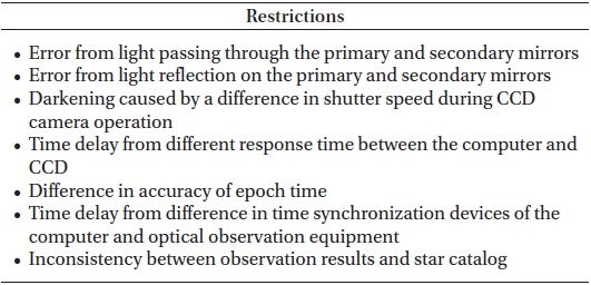
Despite the numerous developments, orbit precision obtained from optical systems are known to be less precise compared to that of radar and laser systems. The restrictions that occur in optical observations are listed in Table 2.
[Table 2.] Restrictions of optical satellite observation.

Restrictions of optical satellite observation.
This study did not perform bias corrections on simulations, but several adjustments were made to account for the restrictions of Table 2 when using actual observation data.
3. UTILIZATION OF ORBIT DETERMINATION TOOL KIT (ODTK)
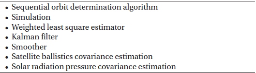
The ODTK program used in simulations is a commercial program for orbit determination developed by AGI and commonly used in orbit analysis simulations or the processing of actual observation data (Hujsak et al. 2007; Vallado et al. 2009). The characteristics of ODTK is shown in Table 3.
[Table 3.] Characteristics of Orbit Determination Tool Kit (Hujsak et al. 2007).

Characteristics of Orbit Determination Tool Kit (Hujsak et al. 2007).
3.2 Observation Data Processing Using ODTK
In the processing of observation data, ODTK supports the initial orbit determination method, least square method, and sequential processing method. Results obtained from the initial orbit determination method are used as
Initial settings, a factor that significantly influences simulation results, must be thoroughly verified. A general configuration is needed for observatory coordinates and dynamic model. The minimum observation altitude angle was set for ground observatories, thus a restriction due to any obstacles near observatories was eliminated beforehand. Obstacle-related restrictions were reduced by setting the minimum observation angle. To ensure a conducive observation environment, it is important to organize the surroundings of optical observatories. The minimum observation limiting angle minimizes the effect of sky brightness, which occurs even when the sun goes below the horizon.
TLE, used for the initial configuration of artificial satellites, can be obtained from the Space-Track. The TLE data applied to simulations is shown in Table 4 (Historical TLE search 2014).
[Table 4.] Six orbital elements of COMS converted from TLE.
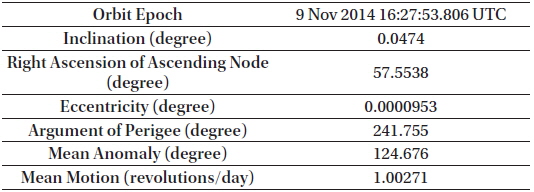
Six orbital elements of COMS converted from TLE.
In ODTK, the force model can be reflected during the initial configuration of satellite orbit. The basic orbit propagator model was HPOP, and in addition, other models such as equatorial motion and arithmetic integration can be applied. The uncertainty of artificial satellite orbits can be adjusted by users to reflect the random distribution of simulations. The gravity model integrates white noise in the gravity field and allows accurate error calculation. For solar radiation pressure, a penumbral cone model based on the earth and moon shadows was applied (Vallado et al. 2010).
4. SIMULATION OF OPTICAL OBSERVATION AND ITS NOISE
4.1 Baseline of Dual Optical Observatory Setup
Roh et al. (2011) assumed that observatory locations were in Korea, India and Australia. Through orbit determination simulations for geostationary satellites, he examined the effects of observation time interval, observation error and number of observation sites. Since most studies based on ground observatories involve a long distance between observatories and satellites, this study selected observatories with long baseline distances. Instead of using data from ground observatories concentrated in a small area, it is more advantageous to obtain data from those with larger baseline distances, even if they are fewer in number.
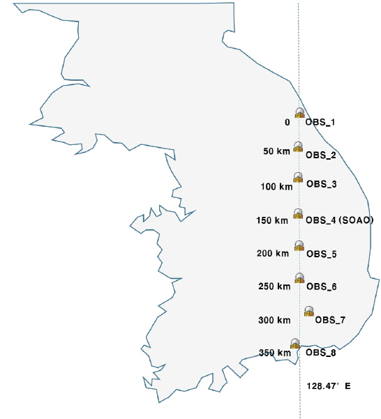
As the topology of the Korean peninsula shows the longitudinal axis is much shorter than the latitudinal axis, we can expect the longer baseline with the latitudinal arrangement of multiple optical observatories. Excluding the southern island populated part, the longitudinal distance of South Korean inland is about 300 km. However, the practically feasible maximum longitudinal distance is less than 200 km due to the geographical and demographical reasons. Thus, we fixed the longitudinal axis arranged the virtual observatories along in latitudinal axis with equal distance of 50 km to get the maximum baseline distance of 400 km.
Vallado & Griesbach (2011) used ODTK and Google Earth to determine the position of observatories and to select observatory sites for simulations. In this study, East longitude 128° 47’, where the Mt. Sobaek observatory of the Korea Astronomy and Space Science Institute is located, was selected as the virtual observatory. Since it is approximately 415 km from the Goseong Unification Observatory to Tongyeong, Gyeongnam Province, the baseline distance of each observatory was set as 50 km for the simplification of simulation. To minimize the observation restriction due to the obstacles around observatories, the locations of the observatories were selected accordingly. This issue was avoided by using Google Earth’s three-dimensional terrain view. Observatories were set up at the coordinates having the maximum altitude within a 500 m radius of the installation site, which was selected to prevent topographical restrictions. A total of 8 virtual observatories were established. Table 5 shows the detailed coordinates and altitude, and Fig. 2 presents the arrangement of observatories.
[Table 5.] The Positions and altitudes of virtual observatories.
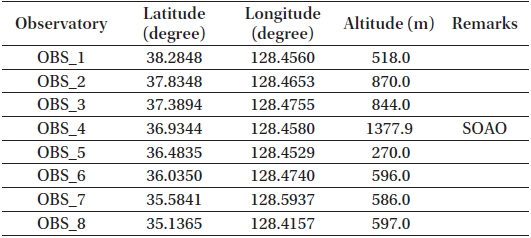
The Positions and altitudes of virtual observatories.
As explained earlier, for geostationary satellites, continuous observations are possible even at night as long as weather permits. The observation time was set from sunrise to sunset, and the observation time interval was one minute. A geostationary satellite moves at a speed of 7.2922×10⁻⁵ rad/sec. To utilize the Star Catalogue, observations must be made using sidereal tracking. For low orbit satellites with relatively short arcs, it is necessary to have a telescope that supports accurate observation analysis.
To maintain its orbit, COMS is subject to correction maneuvers. Two maneuvers are carried out each week for East-West and North-South maintenance. The simulation period was set to avoid any change in orbit. Observation results obtained from one week of observation, from Sunday to Monday, were used in orbit determination.
4.3 Observation Noise Generation
Noise should not be included for precise orbit determination, but actual observation results contain various types of noise. Choi et al. (2011) attempted orbit determination using actual optical observation data and performed a correction for each stage. This study does not require correction since observation data is generated from simulations, but when actual observation data is involved, adjustments have to be made for time synchronization, CCD and other equipment, and WCS.
White noise is in the form of a normal distribution and is widely used because of its mathematical flexibility. The white noise used in ODTK can be expressed as follows. Eq. (1) is the white noise expressed as the Brownian motion, in which [


where, Eq. (2) is the average of white noise, and the sum of all averages is ‘0.’ Eq. (3) is the definition of white noise dispersion.


When calculations are made with Eq. (3) substituted in Eq. (2), white Gaussian noise as expressed in Eq. (4) is obtained, which in turn leads to Eq. (6). Here, k is a constant within
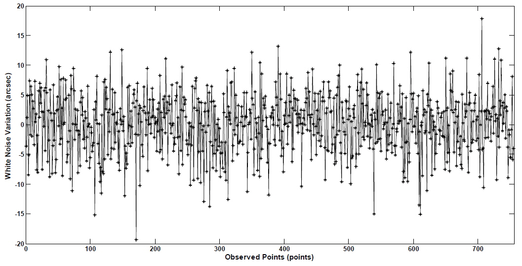
The size of white noise was set as 0 arcsec, 5 arcsec, 10 arcsec, 20 arcsec, 30 arcsec, 40 arcsec, 50 arcsec, and 100 arcsec. After generating observation data for each white noise type, the observation data was verified. The equalities of the numbers of observation points were checked with the simulated observation including 0 arcsec and 5 arcsec white noise cases. Fig. 3 is showing the difference between 5 arcsec and 0 arcsec cases after applying proper simulated noise values for each observation points.
4.4 Multiple Baseline Comparison
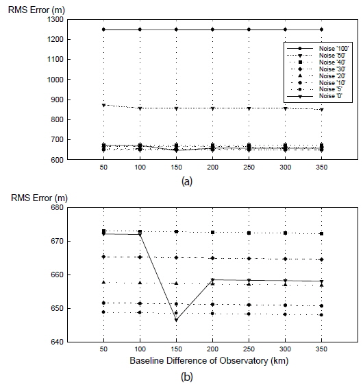
To examine the effects of baseline distance, observation data was classified by baseline distance and limited to those retrieved from two observatories. Since the difference in baseline distance was 50 km, orbit determination simulations were performed 7 times for observatories 1 to 8 over 350 km. Comparisons were made for the radial, in-track and cross-track parameters in the RIC frame, and RMS values were analyzed. In-track parameters are associated with the most change in the RIC frame. The RMS results for in-track parameters are presented in Table 6. The values are highly different according to the white noise amount in the initial 50 km, and show improved precision with larger baseline distance. As you can see in Table 6; Fig. 4, there are small improvements in In-track RMS error of orbit determination as the baseline difference extended from 50 km to 300 km. Also, as the simulated white noise level of observation goes from 100 arcsec to 0 arcsec, In-track RMS error of orbit determination improves significantly as expected. Between 0 arcsec and 40 arcsec of white noise level in simulated observation, In-track RMS error of orbit determination with each white noise level shows very similar values.
[Table 6.] Orbit determination results with 2 observatories (In-track RMS) (unit: meter).
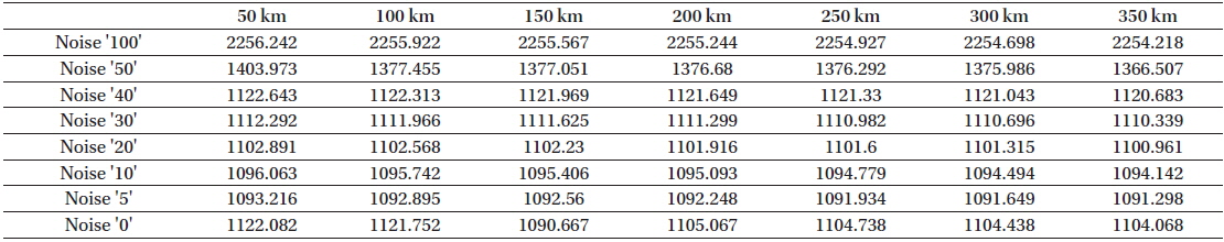
Orbit determination results with 2 observatories (In-track RMS) (unit: meter).
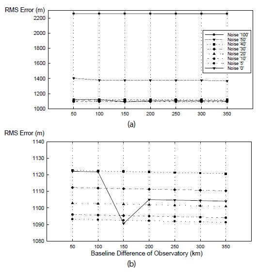
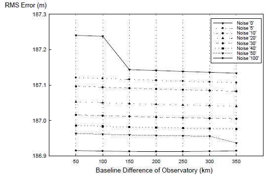
Figs. 5 and 6 shows the radial and cross-track RMS error of orbit determination results respectively. As baseline distance increases, radial and cross-track error show improved precision.
A total of 756 observation points were generated for the observation period of 1 day. Since the limiting Sun angle below the horizon was set as ‘-5’ degrees, sufficient data was generated for orbit determination through simulated observations. It should be noted that actual observations conditions involve more restrictions. The acquisition of an adequately sufficient amount of observation data allowed simulations to be stably performed.
The effects of white noise on orbit determination were examined through simulations. There were eight types of white noise classified from 0 arcsec to 50 arcsec at 10 arcsec intervals. Assuming that correction had been carried out, an additional 5 arcsec was added. The effects of very large white noise were explored by reflecting 100 arcsec of noise in the observation data. Figs. 4-6 show the results by amount of white noise. No significant difference was observed from 0 arcsec to 40 arcsec. On the other hand, 50 arcsec and 100 arcsec of white noise led to very large values. During orbit determination based on actual observation data, it is important to perform corrections for the restrictions of Table 3 to prevent noise from interfering with observation results, which can be regarded as the first step to achieving more precise orbit information.
The effects of baseline distance between observatory stations on precise orbit determination were examined through simulations. In consideration of topographical restrictions, observatories were placed 50 km apart in terms of longitude. As such, the simulations only accounted for the vertical difference between observatories. As presented in Section 4, RMS results are clearly different for each RIC factor. When the baseline distance was 350 km, the RMS results of in-track factors were more accurate by a maximum of 18 m (noise 0 arcsec). Moreover, the radial and cross-track factors also showed improved precision by a few meters over varying amounts of white noise.