Laser ranging techniques are widely used for both industrial and scientific application in contactless measurement as nondestructive testing, in contrast to other measuring technologies that have to contact the target surface [1]. Laser ranging techniques have the potential to improve the productivity of manufacturers and the quality of manufactured products due to their swiftness and high precision.
Heretofore, conventional optical distance measurement methods can technically be put into three categories: interferometry, time-of-flight and triangulation methods [2]. It is undeniable that these traditional methods can exhibit high accuracy, but the applications are limited due to their short unambiguity range determined by the wavelength used [3] or to their complicated experimental setups. Thus, these methods are inappropriate when the measurement is carried out in a narrow space. For example, in consideration of their dimensions, there is not enough space to install devices based on conventional methods for cylinders with inner diameters of less than 10 centimeters.
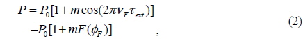
Fortunately, this shortcoming can be overcome by a very interesting coherent technique called self-mixing interferometry (SMI) [4]. The SMI system is simpler than conventional interferometers because many optical elements, such as the beam splitter, reference mirror, and external photodetector, are not required [5]. The self-mixing phenomenon occurs when the laser beam is partially reflected by a target in an external cavity and mixed with the light inside the laser cavity, which results in variation in emitted power and lasing frequency [6]. Information about the motion of the target can be deduced by an integrated phototransistor through analyzing the variation.
The inquiry into distance measurement based on SMI has attracted much attention during the past few decades due to its simplicity, compactness, and low cost [7]. Many methods have been presented which use the linear relation between beat frequency and distance [8-13], such as counting the number of mode hops [8] or utilizing the interpolated FFT [13]. Most signal-processing work has focused on spectrum estimation algorithms until recently, and resultant measurement resolution has been promoted to 0.1 mm [13]. However, in terms of signal-processing theory, inherent drawbacks of the spectrum estimation algorithms such as spectrum leakage will influence the measurement of beat frequency and degrade the accuracy of distance measurement. Moreover, further post processing such as adjustment is often required to extract the accurate frequency [14], which makes the measurement complex.
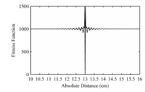
In order to avoid the shortcomings of spectrum estimation algorithms, we propose the use of optimization algorithms to estimate the distance information, which eschews spectrum estimation and searches for the minimum of a fitness function. The fitness function is established based on the SMI signal that contains the distance information. The function is a multimodal function and obtains the sole global minimum that corresponds to the actual distance. Because of this, we can estimate distance by means of searching for this global minimum.
Traditional optimization methods such as Newton’s method and some intelligence algorithms such as the genetic algorithm (GA) [15] and the PSO algorithm [16] can extract absolute distance from the self-mixing signal. Newton’s method is widely used among local searching algorithms due to its fast convergence ability. This method can be utilized if we initialize a certain number of points searching local optima simultaneously in the predicted area, and then find the minimum of all local optimal solutions, thus preventing trapping into local optima. However, the performance of this method depends largely on initialization of points and searching step size, which are difficult to adjust in practical measurements. What is more, the elapsed time of Newton’s method is higher than other optimization methods due to the large number of points. As to intelligence algorithms, we take GA and PSO under consideration, as they have versatility and ability to optimize various kinds of multimodal functions. However, the process of coding should be implemented before calculation, and there are some other complex operations in the genetic algorithm during the calculation, such as crossover and mutation. More parameters should be taken into consideration in comparison with PSO. As a result, we choose PSO to estimate the distance.
The paper is organized as follows: Section II presents the detailed theoretical analysis about self-mixing interferometry and the particle swarm optimization algorithm. Experimental results and comparison with interpolated FFT are discussed in Section III. In Section IV, the influence of different external feedback strength parameter C and an optimal selection of inertia weights are presented. Conclusions are drawn in Section V.
2.1. Self-mixing Interferometry
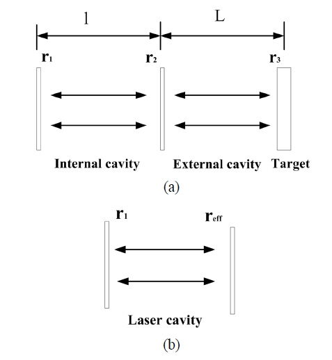
A schematic arrangement for a solitary single-mode laser diode (LD) under external feedback can be represented by a three-facet Fabry-Perot cavity and simplified by a two-facet Fabry-Perot cavity, as shown in Fig. 1.
Here


here
When the sawtooth current is injected into the laser,

here
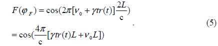
The distance
2.2. Particle Swarm Optimization
The particle swarm optimization is a parallel evolutionary computation technique based on the social behavior metaphor. The PSO algorithm is initialized with a population of random candidate solutions in a predicted area, conceptualized as particles [18]. Each particle is treated as a point to represent an estimated distance and the particles are updated at each iteration. The ith iteration of particles can be represented as
The velocity of each particle is updated according to its current position. The difference between the best position of each particle and the individual’s current position is stochastically added to the current velocity, causing the trajectory to oscillate around the best position of each particle. Simultaneously, the difference between the best position of all particles and the individual’s current position is also stochastically added to the current velocity. Thus, the particle is adjusted to search around the two best positions and all particles get close to global best position [20]. With a sufficient number of iterations, the global best position approximates the actual distance where the fitness function obtains the minimum.
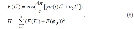
In summary, the


here
The first part of the Eq. (7) is the previous velocity of the particle. The second part represents the private thinking of the particle itself and the third part represents the collaboration among the particles [22]. Thus the new velocity of each particle can be calculated with the contribution of its previous velocity and the distances of its current position from its own best experience (position) and the group’s best experience. Eq. (7) exhibits local search ability without the first part and more likely global search ability by adding the first part. In order to balance the two abilities, an inertia factor

The factor
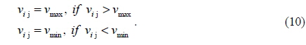
In addition, the velocities of the particles are confined within [vmin, vmax] as in Eq. (10) to guarantee that the particles are confined to searching in forecasted space [24].

PSO has the ability to search global minima working on a population of potential solutions. However, this algorithm has the drawback of time complexity. In practical measurements, the actual distance is unknown and we have to estimate the range of measurement. Because of this, there is large amount of calculation with searching into such a wide range.
In order to decrease the time consumed, we implemented a way to shrink the exploration range [15] before the implement of PSO to accelerate the speed of measurement. During the accelerating, the range of all points will be updated according to the performance of the last iteration of particles. The maximum and the minimum of a fraction of particles ranked in the front to get the best fitness function value will be selected to establish the new range. The particles that give the maximum and the minimum should also be added to the next iteration to avoid the neglect of the actual distance. Because of this, the range will be shrunk to a small range around the actual distance after several iterations of update. After the accelerating, the PSO can find out the global minima within several tens of iterations, which can significantly decrease the time consumed.
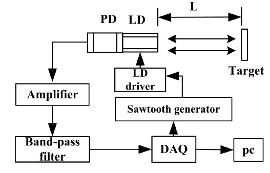
We implemented some experiments to confirm the validity of the PSO algorithm, and the experimental setup is exhibited in Fig. 3.
The VCSEL HVS6003-001 with an integrated phototransistor and a threshold current of 2 mA was utilized in the experiment. It emits a polarized beam with a central wavelength of 850 nm. The VCSEL is driven by a modulated sawtooth current with amplitude 1 mA and frequency 50 Hz, biased at 7 mA. The current is generated by a digital to analogue output channel of NI’s DAQ card.
SMI signal occurs when the laser beam is partially reflected by the diffusive target and mixed with the light inside the laser cavity. The SMI signal can be detected by the built-in phototransistor and transformed into light current and then into voltage signal by a sampling resistance. The voltage signal is digitized and sampled by a DAQ card with sampling rate of 100 kHz after the process of an amplifier and a band-pass filter. A PC running the PSO algorithm was utilized to process the samples. The parameters of the algorithm are exhibited as follows. A recommended choice for constant
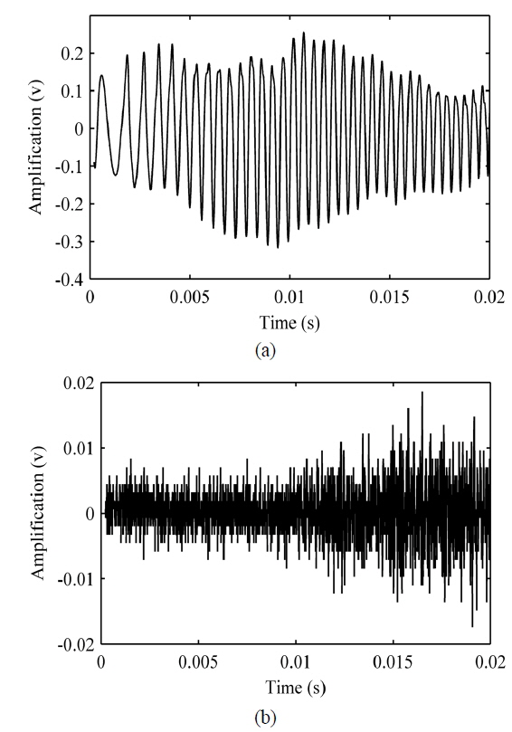
The SMI signal during a modulation period is shown in Fig. 4 (a), the corresponding noise without feedback is shown in Fig. 4 (b). The sinusoidal waveform in Fig. 4 (a) shows that the device works under weak feedback regime (
The target is fixed on a mechanical translator with precision 3
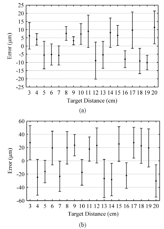
A resolution better than 25 μm in the range from 3 to 20 cm can be seen from Fig. 5 (a) to demonstrate the performance of PSO in processing of the SMI signal. In addition, the results from Fig. 5 illustrate that the PSO algorithm has superiority to interpolated FFT in resolution and stability. This result may be explained by the following reasons. Interpolated FFT suffers from inherent drawbacks such as spectrum leakage, which will influence the measurement of beat frequency and degrade the accuracy of distance measurement. What is more, inapplicability in the condition with dense frequency spectrum will further worsen the measurement. Whereas, the PSO depends on the fitness function that is established from the self-mixing signal. For this matter, PSO is appropriate to realize high resolution and stability in the absolute distance estimation eschewing the difficulty in frequency analysis.
However, PSO performs well at the expense of being time consuming. We processed the same data in MATLAB environment on the PC with dual-core 2.8 GHz CPU and 2 GB RAM. The elapsed time of PSO is nearly 10 s while the elapsed time of interpolated FFT is less than 1 s due to the fast calculation algorithm. Because of the application of accelerating, the elapsed time of PSO has decreased from more than 80 s to nearly 10 s at the same resolution level. Further optimization should be investigated to accelerate the calculation. For example, a simpler fitness function will reduce the amount of calculations, and high seed devices such as FPGA have the potential ability to decrease the time consumed.
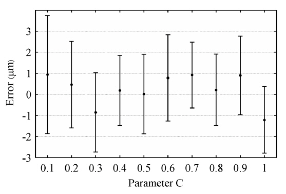
4.1. Influence of External Feedback Strength Parameter C
A single solution for
For a very weak optical feedback level when
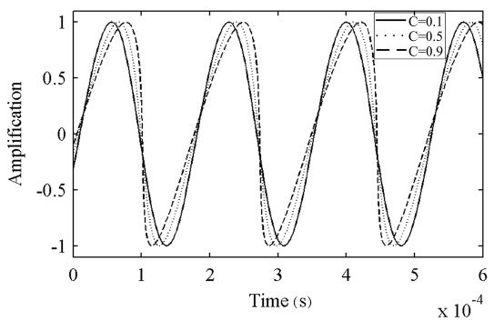
As we can see from Fig. 7, the change of parameter
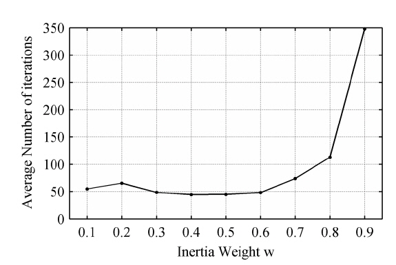
4.2. Parameter Selection of Inertia Weight w
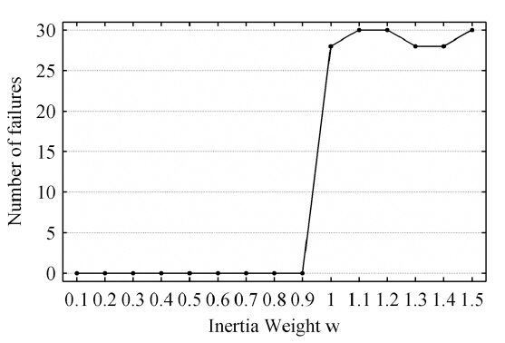
The inertia weight
It is observed that there is no distinct difference in the number of iterations when
In this paper, an approach of SMI based on particle swarm optimization for absolute distance estimation is proposed. The PSO algorithm with an inertia weight was utilized to find the optimal solution of the multimodal fitness function and then to estimate the actual distance value. Some experiments were implemented to demonstrate the validity of this algorithm and the superiority to interpolated FFT in process of SMI signal, and the absolute distance was estimated with a resolution superior to 25 μm in the range from 3 to 20 centimeters. Some simulations with different external feedback strength parameter