The estimation of position and orientation is vital for navigation of a mobile robot. The estimation of location, called localization, has been studied extensively. There are many methods that have been proposed and implemented. These methods include simple dead reckoning, least squares, and other more complicated filtering approaches.
The most intuitive and trivial method, which is also impractical, is dead reckoning. This method integrates the velocity over time to determine the change in robot position from its starting position. Other localization systems use beacons [1–5] placed at known positions in the environment. The beacons use range data to the robot. The range sensors use ultrasonic or radio frequency signals to determine the distances between the robot and the beacons. The least squares method or filtering method uses the range data to estimate the position of the mobile robot. Uncertainty in robot motion and the noise in the range measurement affect the performance of the estimation; additionally, some control parameters of the methods should be adjusted according to the levels of uncertainty and noise. There have been several filtering approaches for localization.
There have been several filtering approaches for localization. Several of the major approaches are the Kalman filter (KF), extended Kalman filter (EKF) [6], unscented Kalman filter (UKF), and particle filter (PF) [7–9]. All of these filters follow the Bayesian filter approach. The variations in the Kalman filter assume that the uncertainties in robot motion and measurement are Gaussian.
The pure KF only uses a linear model of robot motion and sensor measurement. To handle the nonlinearity in robot motion and sensor measurement, the EKF approximates the nonlinearity with a first-order linear model. UKF, a recent development of KF, does not approximate the robot motion and sensor measurement. Instead, it uses a nonlinear model of motion and measurement as it is. It uses samples called the sigma points to describe the probabilistic properties of the robot motion and sensor measurement. UKF also assumes that all the uncertainty involved in the system is Gaussian.
Though EKF has been used widely and successfully for mobile robot localization, it sometimes provides unacceptable results because real data can be very complex, involving elements of non-Gaussian uncertainty, high dimensionality, and nonlinearity. Moreover, EKF requires derivation of a highly complicated Jacobian for linearization. Therefore, Monte Carlo methods have been introduced for localization.
Monte Carlo localization (MCL) is based on a particle filter [10–12]. MCL can solve the global localization and kidnapped robot problem in a highly robust and efficient way. The Monte Carlo localization method uses a set of samples, called the particles, to depict the probabilistic features of the robot positions. In other words, rather than approximating probability distributions in parametric form, as is the case for KFs, it describes the probability as it is using the particles. MCL has the great advantage of not being subject to linearity or Gaussian constraints on the robot motion and sensor measurement.
This paper is concerned with the estimation of robot position and orientation in an indoor environment. We have used a sensor system comprised of static ultrasonic beacons and one mobile receiver installed on the robot. The robot navigates through predefined path points. The exteroceptive measurement information is the range data between the robot and the beacons. In this experiment, we have used a differential drive mobile robot. The paper contributes to understanding the effect of control parameters on the localization performance. How the uncertainty in robot motion and sensor measurement affects the location estimation has been exploited through experiments.
The remainder of this paper is organized as follows. In Section 2, MCL and its fundamentals are discussed. Section 3 illustrates details of the experiment and analysis of MCL. Section 4 covers the discussion of the experiments, and Section 5 concludes the paper.
2. Monte Carlo Localization and its Models
The MCL method iterates sampling and importance resampling in the frame of the Bayesian filter [13] approach for localization of a mobile robot. It is alternatively known as the bootstrap filter [14], the Monte Carlo filter [15], the condensation algorithm [16], or the survival of the fittest algorithm [17]. All of these methods are generally known as particle filters.
MCL method can approximate almost any probabilistic distribution of practical importance. It is not bound to a limited parametric subset of probabilistic distributions as in the case of an EKF localization method for a Gaussian distribution. Increasing the total number of particles increases the accuracy of the approximation. However, a large number of particles degrades the computational efficiency that is needed for real-time application of the MCL. The idea of MCL is to represent a belief about a robot position with a particle set , each representing a hypothesis on the robot pose (
Monte Carlo localization repeats three steps: 1) application of a motion model, 2) application of a measurement model, and 3) resampling of particles. These three steps are explained in Table 1 using pseudocode.
[Table 1.] Monte Carlo localization (MCL) algorithm
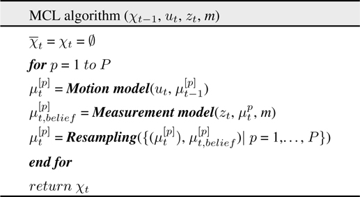
Monte Carlo localization (MCL) algorithm
In Table 1, the prediction phase starts from the set of particles and applies the motion model to each particle in a particle set . In a measurement model, the importance factor, sometimes called the belief of each particle is determined. The information in the measurement
The resulting sample set usually consists of many duplicates. It refocuses the particle set into a region of high posterior probabilities. The particles that were not contained in have lower belief. It should be noted that the resampling process neither includes the particles in order from the highest belief nor excludes the particles in order from the lowest belief. Thus, the set consists of
A motion model is used to predict the pose of the robot from the previous pose using the control command or proprioceptive motion sensing (
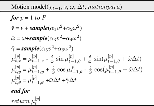
Motion model
In Table 2, , , and constitute a particle that represents the pose of the robot. Δ
In the measurement model, the belief of the predicted particles is computed utilizing the received range information from the beacons. Table 3 shows the proposed measurement model that we have to implement in MCL. is the distance between the predicted particle and the beacons.
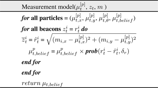
Measurement model
Finally, all particles are resampled, i.e., a new set of particles are drawn from the current set on the basis of the belief . We use systematic resampling, which is also known as stochastic universal resampling because it is fast and simple to implement.
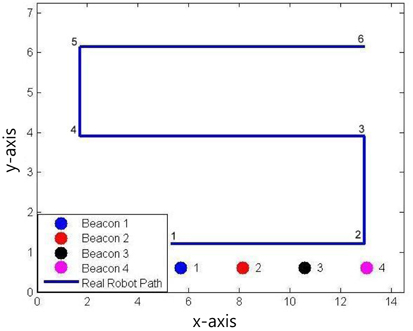
The experiments are conducted in a classroom with chairs and tables on which computers and monitors are located. The four ultrasonic beacons are installed on the ceiling.
Figures 1, 2 shows the experimental setup which indicates the trajectory of the robot motion and the location of ultrasonic beacons. The positions of the beacons and way points are provided in Tables 4 and 5, respectively.
[Table 4.] Locations of the beacons
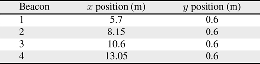
Locations of the beacons
[Table 5.] Locations of the way points
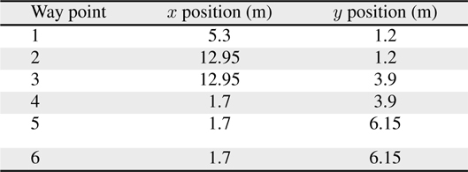
Locations of the way points
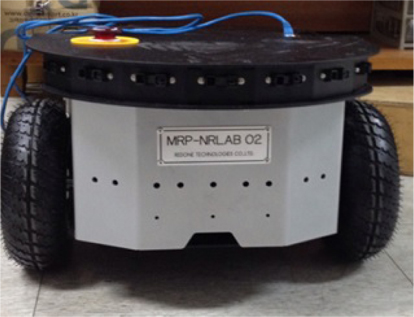
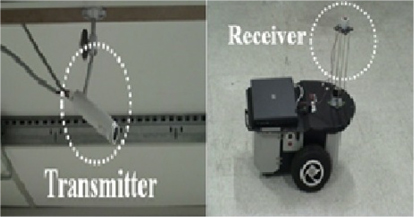
We use the MRP-NRLAB 02 differential drive robot (see Figure 3) manufactured by RED ONE technologies and the USAT A105 ultrasonic sensor system (see Figure 4) from the company Korea LPS. The work area for the experiment is 14.5
The robot is controlled by a joystick and uses the wheel encoder data to calculate the translational velocity
[Table 6.] Control parameter values
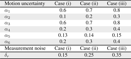
Control parameter values
During the experiment, the ultrasonic range measurement system often fails in detecting some of the ranges. Because of the failure, ambiguity and large estimation error are observed in the path segments from 3 to 4, 4 to 5, and 5 to 6.
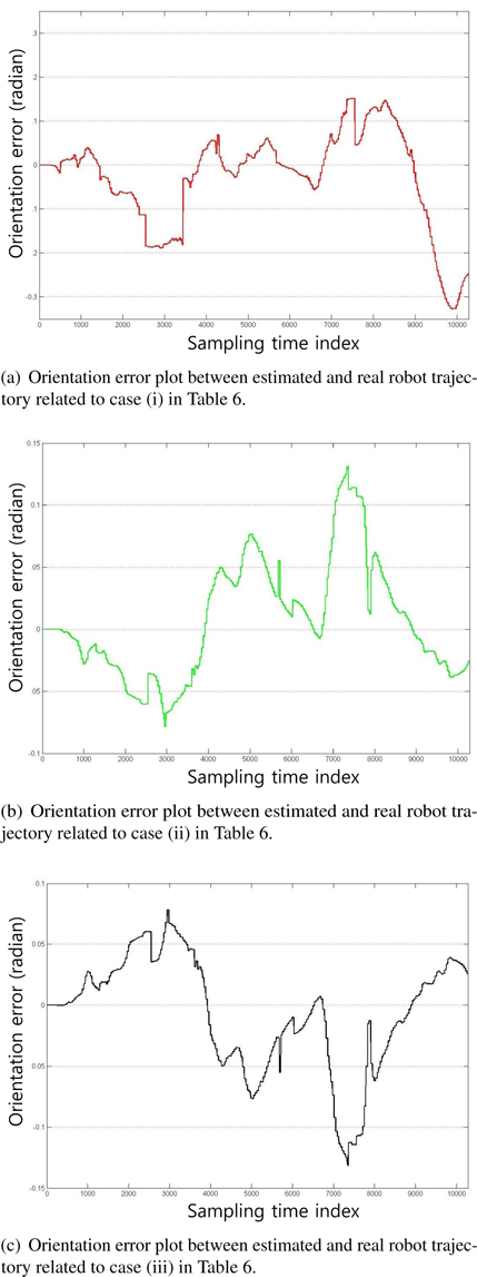
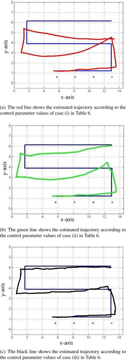
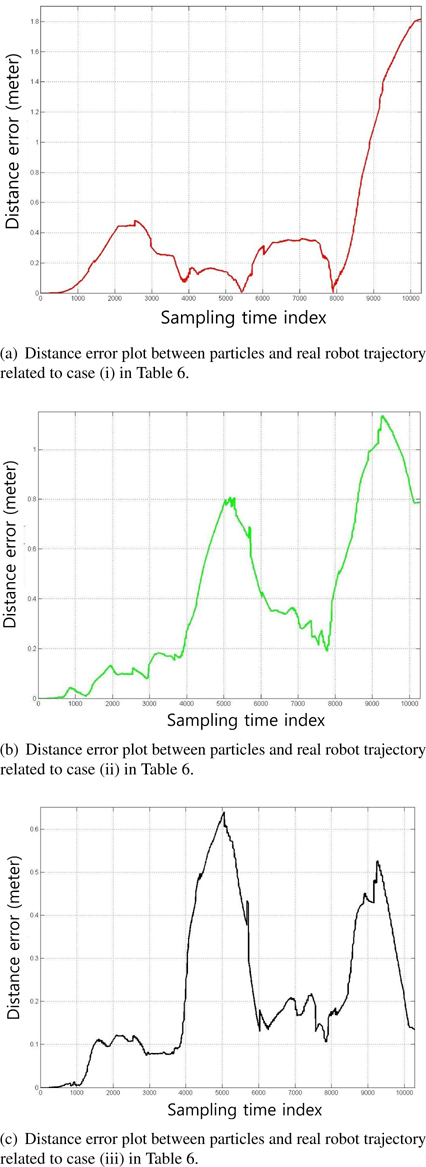
Figure 5 shows the plots of the estimated trajectories by colored lines according to the values of the control parameters, as shown in Table 6. The asterisks represent the positions of the beacons. Figures 6 and 7 illustrate the distance error and orientation error between the estimated and real robot trajectories. Tables 7 and 8 list the mean and standard deviation of the distance error and orientation error of the estimation, respectively. From the experimental results, the estimation error of the robot is observed to decrease when the appropriate control parameter values are used.
[Table 7.] Mean of distance error and orientation error
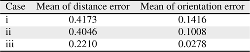
Mean of distance error and orientation error
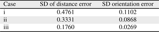
[Table 8.] Standard deviation (SD) of distance error and orientation error

Standard deviation (SD) of distance error and orientation error
A variety of techniques and suggestions have been proposed for mobile robot localization [18–24]. It is evident that a comparison of different techniques was difficult because of a lack of commonly accepted test standards and procedures. We have developed our own experimental environment using four ultrasonic beacons and six way points for robot navigation. An analysis of MCL was performed under three different cases, as provided in Table 6. Each case in Table 6 is categorized according to the low, medium, and high values of motion uncertainty and measurement noise. The investigation of MCL analysis was based on the following:
1) plotting the trajectory of the estimated position against the real robot trajectory,2) calculating and plotting the distance error and orientation error between the real robot position and the estimated position, and3) evaluation of mean and standard deviation of the distance error and orientation error.
Large estimation error is observed in (a) and (b) in Figure 5, which corresponds to cases (i) and (ii), respectively. Figure 5c, which corresponds to case (iii), shows the least estimation error. The results also suggest that the motion error and measurement noise of the experiment are relatively high.
Figures 7 and 8 show the distance error and orientation error for the experiments. The mean and standard deviation of the errors are listed in Tables 7 and 8, respectively. The results are shown in Figures 5 through 7, and Tables 7 and 8 indicate that the proper selection of control parameters is crucial for the use of MCL. MCL fails if the values of the control parameters assume that the uncertainty of robot motion is lower than the actual uncertainty. Likewise, assuming that the measurement uncertainty is lower than that of the actual measurement deteriorates the estimation performance.
This paper shows results of MCL used for localization of a mobile robot in an indoor environment. The experiment uses a differential drive robot, which uses wheel encoder data and range data from four fixed beacons.
The experiments compare three different cases, which represent localization under different control parameter values. The control parameters adjust the uncertainty of robot motion and sensor measurement noise. From the comparison, it is concluded that assuming that the motion uncertainty and measurement noise are lower than the actual values causes poor estimation performance. This is the case for KF approaches, where the mismatch in the process error level and measurement error level causes poor estimation performance.
No potential conflict of interest relevant to this article was reported.