The current trend of face recognition research is toward greater use of three-dimensionl (3D). This trend is due to the rapid evolution of technologies that have enabled the development of image acquisition tools such as 3D scanners and the Microsoft Kinect sensor. In addition, the emphasis of research has moved towards 3D in order to improve performance accuracy of 2D face recognition under difficult conditions. To obtain highly accurate results, appropriate preprocessing steps are needed because their result will affect the results and processes of feature extraction and classification.
Mian et al.[1] have researched automatic 3D face detection, normalization, and recognition. They used data from the face recognition grand challenge (FRGC), which was taken from the Minolta Vivid 900/910 series sensor. The CyberwareTM 3030PS laser scanner was used by Blanz and Vetter [2] to record 3D face data. It was also used as an interactive tool for filling holes and removing spikes. Unfortunately, the price of these data acquisition devices is prohibitive. Although the 3D face data has high resolution [2]; it requires a smoothing process in preprocessing. They used a median filter for the smoothing process. Li et al. [3, 4] used the Microsoft Kinect sensor, which is the cheapest hardware available for 3D face recognition. Resampling and symmetric filling was used for smoothing. Chen et al. [5] used geometric hashing and a sample training set of labeled images as their denoising method. Mean and median filtering are also used for mesh smoothing which has been applied to face data [6]; to get a smooth result, these methods require many iterations. However, to improve the results of the 3D point cloud texture in the preprocessing step, especially using RGBD images, a researcher usually needs the assistance of a 3D face template model [2-4]. When a 3D face template model is used, a fitting method is absolutely necessary. Iterative closest point (ICP) is used to fit a 3D face point cloud to a 3D face template model [3], but this method requires a long computation time. In 3D face recognition [7, 8], an affine transform or homogeneous transform is used to replace the ICP method for fitting [4]. We emphasize that these methods are not very efficient.
Anisotropic diffusion is the method introduced by Perona and Malik [9]. This method is very useful because it is simpler than the others. Anisotropic diffusion can be implemented on 1D, 2D, and 3D data. Gerig et al. [10] used anisotropic diffusion for filtering MRI data where it has been applied to 2D and 3D image data with one or two channels [11, 12]. Linear anisotropic diffusion mesh filtering has also been investigated [13].
Anisotropic diffusion has also been used for geometric surface smoothing [14] and has applications in image processing [15].
In this paper, we propose a smoothing 3D face point cloud method based on modified anisotropic diffusion. We use input data from the Curtin Faces Database [4]. The data are derived from the Microsoft Kinect, which produced red, green, blue, and depth (RGB-D) data. These data have been processed into 6D data. Because the 3D point cloud data is noisy we used the relation between 2D data and 3D point cloud data to process it more easily. To denoise and smooth the 3D point cloud, we used the basic anisotropic diffusion method. However, we were required to modify the original anisotropic diffusion to increase performance because the original anisotropic diffusion could not compute perfectly in our case. Selected vertices have been used to detect the value from vertices.
The contributions of this research are as follows. 1)We have developed an easier way to process 3D face point cloud data that uses the relation between 2D images and 3D object point clouds. 2)We have developed a robust, modified smoothing method, where the output has a smooth texture and the same number of vertices as the input in the smoothing process. Our proposed method could be implemented with the Microsoft Kinect, which is a cheaply priced device for 3D object processing.
The paper is structured as follows: In Section 2, we present the method and approach. In Section 3, performance evaluation and results are described. In Section 4, we present our conclusions.
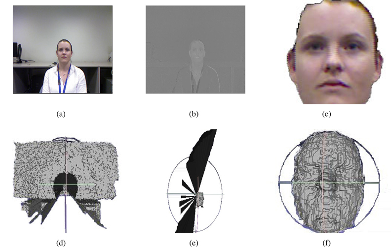
Triangle mesh is one method that can represent a 3D object based upon vertices and face data. This method is simpler than the other; however, we must know about the relationship between vertices and faces. It also requires complex computation to process, if we only use vertices and faces as the information. We propose that the easiest way to process a 3D object point cloud is by using the relation between a 2D image and a 3D object point cloud. Figure 1 shows the result of each step of the cropping process for a 3D face point cloud.
2.1 Point Cloud Reconstruction
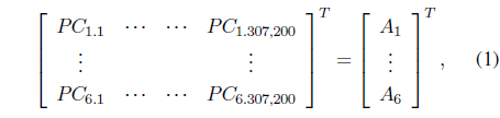
We used a data sample from the Curtin Faces Database [4], which has 307,200 rows and six columns of point cloud matrix data for each subject. For easy calculation, we should rearrange the point cloud matrix to 460 rows and 640 columns, where the first, second, and third columns contain

where
For skin or face detection, we can use existing algorithms such as Lucas-Kanade, Viola-Jones, etc. However, in this experiment, we used a simple method to detect the face in 2D images. We used the YCbCr color format to separate the face from the background. We know that
2.3 3D Face Point Cloud Cropping
The chrominance red layer was converted to the monochrome format for easy cropping of 2D faces. Because the object and environmental conditions are always changing, an adaptive threshold should be used to obtain an optimal result for the black and white color format. To solve this problem, we used the Otsu method to adaptively calculate the threshold. Although the adaptive threshold was already used in this system, the result of this system has some noise. We used a median filter and selected an area to reduce its noise. We used a kernel size of 7 × 7 for the median filter. Although using the median filter caused closing and opening of pixels in the image

where


where
Because

Unfortunately, the result of the extraction process still has some noise. This happens because point cloud

The result usually has range 0 ≤ ≤ 3, 000, depending on the distance when we acquire the data.

Eq. (8) describes
In


where
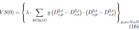
2.4 3D Face Point Cloud Smoothing
Because a 3D face point cloud has nonlinear characteristics, the anisotropic diffusion method has been used to smooth it. Anisotropic diffusion extends isotropic diffusion with a nonlinear term limiting diffusion across boundaries defined by a large gradient in image intensity. In order to enable the isotropic diffusion to preserve features, Perona and Malik [7] modified it.

Eq. (11) describe anisotropic diffusion, where

(12) where


where
In our system, we computed 3D face data like 2D images, so
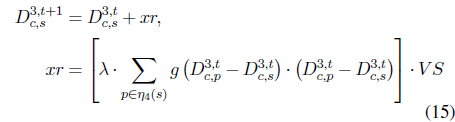

where
3. Performance Evaluation and Result
We tested the proposed method using data from the Curtin Faces database. In this system, we propose three scenarios to investigate the method. The first scenario is a performance comparison of smoothing using five different angles as an input. The second scenario is a performance comparison of smoothing using five different faces, but the same angle as an input. The last scenario is to investigate the performance of smoothing by iteration. The processes were carried out on a 2.4 GHz Intel core i3 processor with 2 GB memory.
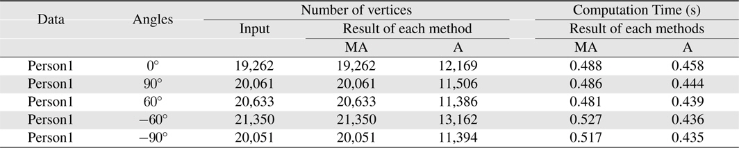
In this experiment, we compared our proposed method and the original anisotropic diffusion method. In the first scenario, the subject was one female face posed at various angles. The angles that we used in this experiment were 0°, 60°, ―60°, 90°, and ―90°. Table 1 shows the simulation result for 0°, 60°, ―60°, 90°, and ―90°. From this table, modified anisotropic diffusion substantially improves the original anisotropic diffusion performance at all angles. Our proposed method can maintain the same number of vertices input in the smoothing process. The computation time of our modified anisotropic diffusion and the original anisotropic diffusion is almost the same; there is no significant difference between the methods.
[Table 1.] Results of comparison methods with different angles

Results of comparison methods with different angles
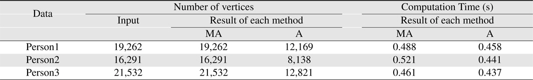
In the second scenario, we used two females and one male face, all posed at the same angle. We used a 0° angle in this experiment. Table 2 shows that modified anisotropic diffusion also can maintain the same number of vertices input in the smoothing process. Both methods have almost the same computation time; there is no significant difference between our modified anisotropic diffusion and the original anisotropic diffusion.
[Table 2.] Results of comparison methods with different faces

Results of comparison methods with different faces
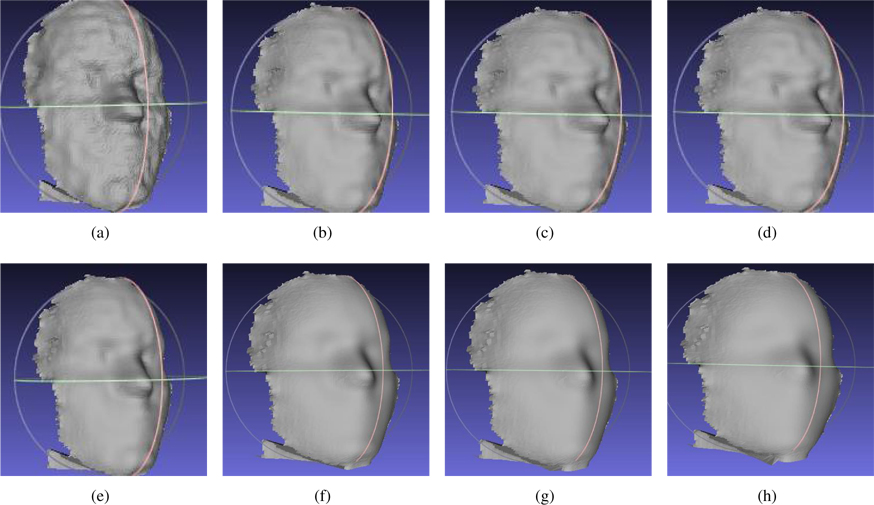
We also investigate the influence of iteration on smoothing process. We used the follow number of iterations at each stage of our experiment: 2, 4, 6, 8, 10, 20, 30, and 40. Figure 2 shows the results from our experiment. From these results, we can see that when the number of iterations was less than 10, the result still left some noise in the texture of 3D face point cloud. A smooth result was only reached when the number of iterations exceeded 10. Unfortunately, these smooth results could cause the disappearance of some features in the 3D face point cloud.
The number of iterations that produced smooth texture in the 3D face point cloud while preserving its features is 10. In 10 iterations, we can still can see features from the 3D face point cloud such as the eye, nose, and mouth regions.
We have presented a modified anisotropic diffusion for smoothing a 3D face point cloud. The key idea of our research is how to smooth 3D face point clouds, the results of which must have the same shape as the original input smoothing and also have the same number of vertices. We have demonstrated that our modification method is more robust than the original anisotropic diffusion. Our method maintains the same shape and number of vertices as the original input in the smoothing process.
Our method is more robust than the original anisotropic diffusion because we modified it by selecting vertices which have values that could not be computed perfectly in anisotropic diffusion. Different faces and different angles in the 3D face point cloud did not influence our system. Our result still has the same shape and number of vertices. There are also no significant differences between the computation times of our modified anisotropic diffusion and the original anisotropic diffusion. The optimal number of iteration is 10 because it will produce a smooth result and preserve the appearance of 3D face point cloud features.