검색 전체 메뉴
PDF
맨 위로
OA 학술지
Study of Ultra-Small Optical Anisotropy Profile of Rubbed Polyimide Film by using Transmission Ellipsometry
  • 비영리 CC BY-NC
  • 비영리 CC BY-NC
ABSTRACT
Study of Ultra-Small Optical Anisotropy Profile of Rubbed Polyimide Film by using Transmission Ellipsometry
KEYWORD
Ultra-small optical anisotropy , Transmission ellipsometry , Anisotropy profile , Rubbed polyimide , Alignment layer
  • I. INTRODUCTION

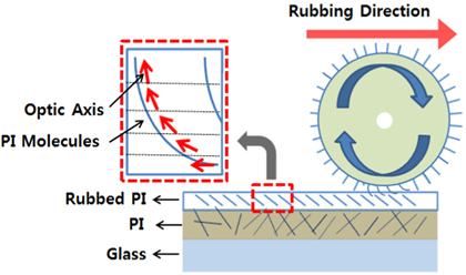
    Rubbing is the process to make an alignment layer, which dictates the molecular arrangement of the liquid crystals (LC) of a liquid crystal display (LCD). In the process, cured polyimide (PI) films are rubbed with a velvet cloth and the surface state of this rubbed PI alignment layer governs the molecular arrangement of the LC, and hence directly affects color gamut and response time of the LCD. For these reasons, a lot of research has been carried out to understand the actual alignment mechanism of rubbing. To characterize the rubbed alignment layers, the precise surface sensitive techniques such as AFM (Atomic Force Microscopy), GIXS (Grazing Incidence X-ray Scattering) or NEXAFS (Near-Edge X-ray Absorption Fine Structure) are often engaged. One possible interpretation of the alignment mechanism of rubbing is the induced alignment by microgrooves [1-4] and another concept for the interpretation is alignment through the reordering of the long-chain organic molecules on the rubbed surface[5, 6]. Optical techniques are commonly applied to characterize the rubbing effect. However, most optical techniques are applied after LC injection since the optical anisotropy of the rubbed alignment layer is too small to be detected using conventional optical techniques [7-9]. In order to characterize the optical anisotropy of the rubbed PI surface itself, a polarization sensitive optical technique such as ellipsometry is used [3, 6, 10-17]. The frontier work of ellipsometric characterization was reported by Hirosawa. [10-12] In analyzing the ellipsometry data, Hirosawa adopted the model that the rubbed polyimide film is composed of a molecularly oriented upper layer and a random lower layer. He found that the thickness of the upper layer ranged from 12.0~13.5 nm and the tilt angle of the principle dielectric axis of the molecularly oriented upper layer was about 40 degrees. The tilt angle varies from 39 degrees to 53 degrees as the rubbing strength is varied, and it increased up to 67 degrees as the rubbed polyimide film is annealed [10-12]. Yang et al. used AFM to determine the mean depth (7.0 nm) of the rubbed PI layer. The mean depth was used to get an optical birefringence of that layer and they reported the birefringence as Δn = 0.17 [3]. The successive reports by Hirosawa et al. reveal that the thickness of the anisotropic upper layer is 36.1 nm for the actual panel, which is much greater than the previously reported one and it remains unchanged even when the rubbing strength is increased. When soaked in solvent, it decreases from 35.6~45.0 nm to 27.1~34.4 nm. The optical birefringence of a strongly rubbed polyimide and that of the weakly rubbed polyimide are reported as Δn = 0.05 and 0.018, respectively [14-16].

    Since it is not the bulk anisotropy but the surface anisotropy of the rubbed polyimide that governs the alignment of LC, finding the optical anisotropy distribution of the aligned molecules of the rubbed polyimide from the surface is very important. Hence the Hirosawa’s model, which uses a very simplified assumption that the surface of rubbed PI is a uniform anisotropic layer, needed to be modified. Meanwhile, a method to determine the optical anisotropy distribution has been reported already for a wide view (WV) film. It is reported that the optic axis of discotic liquid crystals in a WV film is distributed in the form of an exponential function, from the direction normal to the film surface to the direction parallel to it [18, 19]. However, since the magnitude of optical anisotropy of the rubbed polyimide is less than 1/100 of that of the WV film, one has to measure the ultra-small optical anisotropy extremely accurately in order to get the anisotropy distribution of the rubbed polyimide. In this work, we report that the same method which is used to determine the optic axis distribution of discotic liquid crystals in a WV film can be applied to determine the anisotropy distribution of the rubbed PI, when the measurement of very small optical anisotropy is made [17].

    II. MODEL AND THEORY

       2.1. Polarization Analysis of a Non-Uniform Optically Anisotropic Film

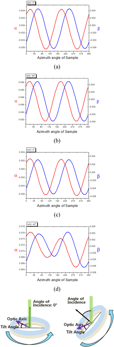
    In relation with the rubbing direction of a rotating roller, organic molecules are expected to distribute as shown in Fig. 1 schematically. The optic axis of organic molecules is also expected to have the same distribution.

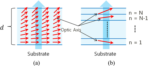
    The change of polarization state of light after transmitting a non-uniform uniaxial film can be described by adopting the method which is used to determine the non-uniform optic axis distribution of discotic liquid crystals in a WV film [18-20]. We first replace the non-uniform uniaxial film in which the optic axis changes continuously, by a stack of N (the number of sub-films) sub-films, each of which is optically anisotropic but spatially uniform, and then calculate the change of polarization state of light after transmitting these N sub-films. If N increases, the polarization state of light after transmitting these N sub-films will approach that of the non-uniform uniaxial film. With the extended Jones matrix formalism, the polarization state of transmitting light can be written as:

    Here, and are Jones vectors representing the polarization state of the transmitting light and that of the incident light, respectively, and is a Jones matrix representing the change of polarization state by N anisotropic sub-films. The explicit expression of this Jones matrix appears below:

    In the above equation, the subscripts e and o represent extra-ordinary ray and ordinary ray, s and p represent s-wave and p-wave, kez and koz in the layer matrix represent z-component of extra-ordinary ray wave vector and that of ordinary ray wave vector, respectively, and d is the thickness of the film. The subscripts at the bottom of each interface and layer matrix represent the numbers of the corresponding sub-films (1, 2, …, N) or the corresponding mediums (air, v1, ..., vn-1), Since the transmission coefficients at the interface between two anisotropic media are not known, we insert a virtual isotropic medium of thickness zero at each interface. Each component of the matrix expressing the polarization state change at this interface between the virtual isotropic medium and the uniaxial medium represents the transmission coefficient at the interface. Thus, for an example, tse of is the transmission coefficient when incident wave from the Nth sub-film is e-wave and the transmitted wave to the air is s-wave. Similarly, top of is the transmission coefficient when the incident wave from the N-1th virtual medium is p-wave and the transmitted wave is o-wave in the Nth sub-film. is the layer matrix representing the polarizing action of the Nth sub-film. The effect of multiple reflections inside the virtual isotropic medium of thickness zero is properly included into the matrix . [18]

       2.2. Rotating Analyzer Ellipsometer and Ellipsometric Constants

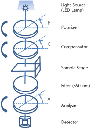
    In PCSA configuration as shown in Fig. 3, the polarization state of light after passing through polarizing devices and sample can be written as shown in Eq. (3). In Eq. (3), the notation suggested by Azzam and Bashara is adopted [21, 22]:

    Here, , is the rotation matrix, and is the Jones matrix representing the polarizing action of the non-uniform, anisotropic sample. The explicit expression of appears in Eq. (2). is the Jones matrix of compensator and A, C, and P represent the azimuth angle of analyzer, that of compensator, and that of polarizer, respectively.

    The intensity of light can be obtained by taking the absolute square of . It becomes a sinusoidal function of the analyzer azimuth angle A. For the rotating analyzer type ellipsometer, A=ωt and the intensity of light is expressed as appearing in Eq. (4), where ω is the angular velocity of rotating analyzer [21, 22]. Since Fourier coefficient α and β in Eq. (4) contain information of the optical anisotropy and its distribution of the rubbed PI, one can determine the optical anisotropy and its distribution by analyzing the Fourier coefficient α and β. [17-20, 23]

       2.3. α, β Variations Versus Sample Rotation Angle of an O-plate at the Incident Angles of 0 Degrees and 40 Degrees

    For a uniaxially anisotropic sample, the variation of the polarization state of transmitted light versus the azimuth angle of the sample strongly depends on the incident angle. For example, if light is incident normal to the surface of an o-plate, then the ellipsometric coefficients α and β versus the azimuth angle of sample show the sinusoidal variation with 180 degree period, as shown in Figs. 4(a) and (c). Figure 4(a) shows the variation of the ellipsometric constants α and β of an o-plate when the tilt angle θ of the optic axis is 0 degrees (i.e., a-plate) and Fig. 4(c) shows it when θ is 40 degrees. The amplitude of the sinusoidal variation of either α or β in Fig. 4(c) is the same as that in Fig. 4(a) multiplied by cosθ. From the analysis of the ellipsometric constants in Figs. 4(a) and (c), when the light is incident normal to the sample surface, one can determine only the combined effect, that is, cosθ multiplied by the magnitude of optical anisotropy, but one cannot determine the magnitude of optical anisotropy and the tilt angle θ, separately.

    If the sample surface is inclined, then the light is incident on the sample surface at an oblique angle, and the angle of incidence is the same as the inclined angle of the sample. The periodicity of measured ellipsometric constants is dependent on the tilt angle θ. When θ is 0 degrees (a-plate), then ellipsometric constants α and β still show the sinusoidal variation with 180 degree period as shown in Fig. 4(b). However, if θ is not 0 degrees, then the sinusoidal variation is distorted and the 180 degree periodicity disappears, as shown in Fig. 4(d) for θ =30 degrees. From these figures, it can be understood that one can determine the tilt angle of the optic axis by analyzing ellipsometric constants obtained at an oblique angle of incidence. Furthermore, if the tilt angle has a distribution like the one in Fig. 2, then ellipsometric constants will not show the 180 degree periodicity and distortion of the sinusoidal variation will be even different from that in Fig. 4(d). The prime subject of this report is to find out both the magnitude and the distribution of the optical anisotropy of the alignment layer by analyzing the variation of ellipsometric constants obtained with and without inclination of the sample. The results are reported in terms of the thickness, the ordinary index of refraction and the extra-ordinary index of refraction of the uniaxial film. The azimuth angle of optic axis together with the distribution of the tilt angle of optic axis is also included.

    III. SAMPLE PREPARATION AND MEASUREMENT

       3.1. PI Coating and Rubbing

    The alignment layer is made on an ITO glass substrate by spin coating. The size of ITO glass is 25×25×0.5 mm3. The solution containing polyamic acid (Nissan 7492k) is coated on the substrates by using a spinning coater. Imidization is performed by curing at 250℃ for 60 min after prebaking at 80℃ for 15 min. Then the films on the ITO glass substrates are rubbed. The diameter of rubbing roller is 30 mm, the rotation speed of the roller is 1000 rpm, the stage speed is 25 mm/s, and the rubbing depth is 0.3 mm. The number of rubbing is two for all samples.

       3.2. Measurement System

    In order to find out the distribution of the ultra-small optical anisotropy whose total retardation is only 0.2~0.4 nm, the precision of the optical anisotropy measurement should be very high. This high precision measurement is achieved utilizing the improved transmission type ellipsometer whose precision to measure a retardation is 3σ < 0.005 nm. The major improvements made to this ellipsometer are, i) the structure of the ellipsometric system is changed from the conventional sample rotation type to the module rotation type, in which the polarizer module rotates while the sample is fixed, ii) the light source is replaced by one which emits a more stabilized light and therefore reduces the background noise level of the system, iii) the rotating polarizer module is synchronized with the rotating analyzer module very accurately, and iv) the tiny background optical anisotropy occurring in connection with the rotating modules is properly compensated [17]. In addition, we installed a dual-rotating sample stage onto this ellipsometer, thus one can set the incline angle of the sample from 0 to 60 degree up to the precision of 0.01 degree, and at the same time one can measure ellipsometric constants as a function of azimuth angle of the rotating sample. We also synchronized the zero point of the rotational sample stage with the rotating polarizer module and the independently rotating analyzer module simultaneously to get ellipsometric data as fast as 15 seconds per sample rotation.

    IV. RESULTS

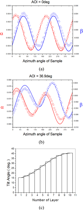
    The measured ellipsometric constants of the rubbed PI sample are shown in Fig. 5, as open circles and open squares. The best fit ones obtained after model analysis are presented as solid lines. Figure 5(a) shows the graphs of α (open squares) and those of β (open circles) when the incidence angle is zero. Both α graph and β graph show the sinusoidal variation with 180-degree period. From the amplitude of this sinusoidal variation, one can get the in-plane magnitude of the optical anisotropy (the optical anisotropy multiplied by cosθ). Also the peak position of this sinusoidal variation indicates the azimuth angle of the optic axis. The in-plane optical anisotropy and the azimuth angle are very useful for the model analysis of the variation of α and β measured at the incident angle of 40 degrees. The measured α and β at 40 degrees of incidence angle appear in Fig. 5(b). From the non-periodic variation of α and β, the optical anisotropic distribution is obtained as follows. We first varied the ordinary refractive index no, the extra-ordinary refractive index ne and thickness d of the rubbed PI film to find the optical birefringence Δn multiplied by d, or Δnd which yields the observed amplitude of the sinusoidal variation in Fig. 5(a). This Δnd is the upper limit of in-plane optical anisotropy. Then no, ne and d as well as other model parameters like θbottom and θtop in Eq.(5) are input into the model analysis as seed values of fitting parameters. After the linear regressional analysis where the calculated ellipsometric constants closest to the measured ones at the incident angle of 0 degrees and the measured ones at 40 degrees are sought, the best fit values of model parameters are determined. The results are summarized as i) no and ne are 1.732 and 1.743, respectively, ii) the thickness of the rubbed PI film is 38.8 nm, iii) the incident angle is 36.9 degree, and iv) the tilt angle of the optic axis is distributed as given by the following equation, with θbottom=14.7°and θtop=40.6°, (see Table 1).

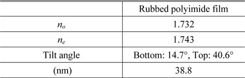
    [TABLE 1.] The summarized optical anisotropy of the rubbed PI film

    label

    The summarized optical anisotropy of the rubbed PI film

    It might be possible that the tilt angle of the optic axis is expressed by a function other than Eq. (5). [18] But exponential ones or trapezoidal ones turned out to fit worse than the sinusoidal one in Eq. (5), only this best-fit tilt angle distribution is presented in Fig. 5(c). The optical birefringence (Δn =0.011) and the thickness of aligned layer (d=38.8 nm) is comparable to the previously reported values. [6-16] The incident angle (36.9 degrees) is a few degrees off from the incident angle set in the measurement system. This deviation is due to the fact that the measured ellipsometric constants are precise but they are not accurate enough and too many strong correlated parameters are used to get the best fit numbers in the model analysis. We expect that the accuracy of our model analysis will be enhanced when we further improve the accuracy of the ellipsometer and when we reduce the number of model parameters by fixing a few parameters(e.g., no and ne) at the numbers determined independently.

    V. CONCLUSION

    The transmission ellipsometric constants of a rubbed polyimide film versus the sample rotation angle are obtained at a normal incidence and at an oblique angle of incidence. The latter ones show a distorted sinusoidal variation. The magnitude of the optical anisotropy of this rubbed polyimide film and the distribution of the optical anisotropy are expressed in terms of the ordinary refractive index (no=1.732), the extra-ordinary refractive index (ne= 1.743), the thickness of rubbed polyimide film (d=38.8 nm) and the cosine-shaped tilt angle distribution of the optic axis with θbottom=14.7° and θtop=40.6°.

참고문헌
  • 1. Kim Y. B., Olin H., Park S. Y., W. Choi J., Komitov L., Matuszczyk M., Lagerwall S. T. 1995 “Rubbed polyimide films studied by scanning force microscopy,” [Appl. Phys. Lett.] Vol.66 P.2218-2219 google cross ref
  • 2. Zhang K., Liu N., Twieg R. J., Auman B. C., Bos P. J. 2008 “Pretilt study of double-layer alignment film (DLAF),” [Liquid Crystals] Vol.35 P.1191-1197 google cross ref
  • 3. Yang F., Zoriniants G., Ruan L., Sambles J., R. 2007 “Optical anisotropy and liquid-crystal alignment properties of rubbed polyimide layers,” [Liquid Crystals] Vol.34 P.1433-1441 google cross ref
  • 4. Yu K.-Y., Lee C.-R., Lin C.-H., Kuo C.-T. 2013 “Controllable pretilt angle of liquid crystals with the formation of microgrooves,” [J. Phys. D: Appl. Phys.] Vol.46 P.045102 google cross ref
  • 5. Stoehr J., Samant M. G., Cossy-Favre A., Diaz J., Momoi Y., Odahara S., Nagata T. 1998 “Microscopic origin of liquid crystal alignment on rubbed polyimide surface,” [Macromolecules] Vol.31 P.1931-1946 google
  • 6. Hirosawa I., Sasaki N., Kimura H. 1999 “Characterization of molecular orientation of rubbed polyimide film by grazing incidence x-ray scattering,” [Jpn. J. Appl. Phys.] Vol.38 P.L583-L585 google
  • 7. Yu C., Bae J., Keum C, M., Lee S. D. 2010 “Optical anisotropy of aligned pentacene molecules on a rubbed polymer corresponding to the electrical anisotropy,” [Current Applied Physics] Vol.10 P.64-67 google cross ref
  • 8. Kimura M., Hasegawa G., Sakamoto H., Akahne T. 2006 “Evaluation of LCD device parameters and rubbed surface of Polyimide by means of renormalized spectroscopic ellipsometry,” [IMID] P.1715-1718 google
  • 9. Sapich B., Stumpe J., Gerus I., Yaroshchuk O. 2000 “Photoinduced anisotropy and LC photoalignment properties of polyvinylcinnamate,” [Mol. Cryst. and Liq. Cryst.] Vol.352 P.9-18 google cross ref
  • 10. Hirosawa I. 1996 “Method of characterizing rubbed polyimide film for liquid crystal display devices using reflection ellipsometry,” [Jpn. J. Appl. Phys.] Vol.35 P.5873-5875 google cross ref
  • 11. Hirosawa I., Sasaki N. 1997 “Influence of annealing on molecular orientation of rubbed polyimide film observed by reflection ellipsometry,” [Jpn. J. Appl. Phys.] Vol.36 P.6953-6956 google cross ref
  • 12. Hirosawa I. 1997 “Relation between molecular orientation and rubbing strength observed by reflection ellipsometry,” [Jpn. J. Appl. Phys.] Vol.36 P.5192-5196 google cross ref
  • 13. Tanooka D., Itoh S., Hirosawa I. 1999 “New characterization technique for rubbed polyimide film for liquid crystal display,” [Jpn. J. Appl. Phys.] Vol.38 P.6454-6455 google cross ref
  • 14. Hirosawa I., Matsushita T., Miyairi H., Saito S. 1999 “Effect of soaking in solvents on molecular orientation of rubbed polyimide film,” [Jpn. J. Appl. Phys.] Vol.38 P.2851-2855 google cross ref
  • 15. Hirosawa I., Miyairi H., Matsushita T., Saito S. 2001 “The relation between pretilt angle of liquid crystal and optical anisotropy of alignment layer,” [Mol. Cryst. and Liq. Cryst.] Vol.368 P.565-571 google cross ref
  • 16. Itoh S., Hirosawa I. 2001 “Observation of an optical anisotropy of rubbed polyimide film on actual LCD panel,” [Mol. Cryst. and Liq. Cryst.] Vol.367 P.745-752 google cross ref
  • 17. Lyum K., H., Park S., U., Yang S., M., Yoon H., K., Kim S., Y. 2013 “Precise measurement of ultra small retardation of LCD alignment layer using improved transmission ellipsometry,” [Korean J. Opt. Photon. (Hankook Kwanghak Hoeji)] Vol.24 P.77-85 google cross ref
  • 18. Ryu J. W. 2010 Ph. D. Thesis google
  • 19. Ryu J. W., Kim S. Y., Kim Y. K. 2010 De“Determination of the optic axis distribution of a hybridly aligned discotic material for wide-view films,” [J. Korean Phys. Soc.] Vol.57 P.233-239 google cross ref
  • 20. Ryu J. W., Kim S. Y., Kim Y. K. 2010 “Polarization analysis of light passing through non-uniform uniaxial media,” [Korean J. Opt. Photon.] Vol.21 P.161-167 google cross ref
  • 21. Azzam R. M. A., Bashara N. M. 1977 Ellipsometry and Polarized Light, Chapter 3 google
  • 22. Kim S. Y. 2000 Ellipsometry, Chapter 3 google
  • 23. Kim H. R., Kim S. Y. 2009 “Precise measurement of optical anisotropy of rubbed polyimide on patterned glass and its nanoscale variation,” [Korean J. Opt. Photon. (Hankook Kwanghak Hoeji)] Vol.20 P.281-287 google cross ref
이미지 / 테이블
  • [ FIG. 1. ]  Schematic figure shows the distribution of organic molecules and optic axes in relation with the rubbing direction of rotating roller.
    Schematic figure shows the distribution of organic molecules and optic axes in relation with the rubbing direction of rotating roller.
  • [ FIG. 2. ]  In calculating the polarization state change after transmitting a non-uniform anisotropic film, the non-uniform film such as (a) is replaced by N uniform sub-films as (b).
    In calculating the polarization state change after transmitting a non-uniform anisotropic film, the non-uniform film such as (a) is replaced by N uniform sub-films as (b).
  • [ FIG. 3. ]  A schematic figure of the improved PCSA type transmission ellipsometer, where the polarizer module and the analyzer module are rotated independently.
    A schematic figure of the improved PCSA type transmission ellipsometer, where the polarizer module and the analyzer module are rotated independently.
  • [ FIG. 4. ]  Simulated variations of the ellipsometric constants α, β of an o-plate, whose Δnd is 0.39 nm. The tilt angle of the optic axis θ is either 0 degrees ((a), (b)) or 30 degrees ((c), (d)). The angle of incidence is either 0 degrees ((a), (c)) or 40 degrees ((b), (d)).
    Simulated variations of the ellipsometric constants α, β of an o-plate, whose Δnd is 0.39 nm. The tilt angle of the optic axis θ is either 0 degrees ((a), (b)) or 30 degrees ((c), (d)). The angle of incidence is either 0 degrees ((a), (c)) or 40 degrees ((b), (d)).
  • [ FIG. 5. ]  Measured ellipsometric coefficients α, β of alignment layer (circles and squares) and the best fit curves (solid lines) when (a) AOI = 0 deg, (b) AOI = 36.9 deg. (c) The best fit distribution curve of tilt angle θ.
    Measured ellipsometric coefficients α, β of alignment layer (circles and squares) and the best fit curves (solid lines) when (a) AOI = 0 deg, (b) AOI = 36.9 deg. (c) The best fit distribution curve of tilt angle θ.
  • [ TABLE 1. ]  The summarized optical anisotropy of the rubbed PI film
    The summarized optical anisotropy of the rubbed PI film
(우)06579 서울시 서초구 반포대로 201(반포동)
Tel. 02-537-6389 | Fax. 02-590-0571 | 문의 : oak2014@korea.kr
Copyright(c) National Library of Korea. All rights reserved.