Recently, software-defined networks that can provide practical ways of handling multi-standard environments have been investigated extensively [1, 2]. In a similar way, software-defined optical receivers are under development in optical fiber communication systems to satisfy many different kinds of modulation formats and baud rates [3, 4]. Although coherent optical systems have become more practical than during their early stages, currently deployed optical transmission systems are mostly the intensity-modulated and direct-detection (IM/DD) type.

Conventional optical receivers for IM/DD systems use a single data per single bit for the decision [5] and require clock recovery circuits. If we could use multiple data for the decision, we do not need the clock recovery circuits [4] while enhancing the receiver sensitivities. However, there are no analyses, to our knowledge, about the correlations between two adjacent data from an optical receiver.

In this paper, we propose to use correlations of two adjacent data for the decision in direct-detection optical receivers. Using the receiver eigenmodes [6-12], we derive the joint characteristic function (JCF) for two successive data from an optical receiver and evaluate the corresponding joint probability density function (JPDF) [13]. The receiver eigenmodes can describe accurately the effects of the amplified spontaneous emission (ASE), received optical waveforms, and shapes of optical and electrical filters within the receiver [7]. Recently, receiver eigenmode contributions have been analyzed as a function of time for the optical receiver output [12]. It has been found that, in conventional dense WDM systems [14-17], where the channel spacing is comparable to the bit rate, the lowest-order (0-th) receiver eigenmode contributes dominantly. We will use this fact to find the correlations of two adjacent data and the threshold line for the decision to get higher sensitivities than conventional receivers.

Before the derivation of the JPDF, we derive the JCF first. We will consider two adjacent samples at times t₁ and t₂. Considering only the polarization component parallel to the received optical signal, we can find the voltage at t₁, denoted as y₁, as [7]

where S_m (t₁) and N_m (t₁) are complex numbers that represent the signal and the noise amplitudes, respectively, for the m-th receiver eigenmode. λ_m is the m-th eigenvalue and k is a proportional constant. For all m, the real and the imaginary parts of N_m(t₁) are mutually independent zero mean Gaussian random variables having an identical variance of In conventional dense WDM systems, the lowest-order receiver eigenmode contributes dominantly [12] and we can approximate

We normalize y₁ such that it becomes a power ratio such that

where the denominator is the noise power per receiver eigenmode per polarization. Similarly, we have the normalized voltage at t₂ as

N₀(t₁) and N₀(t₂) are related by a correlation function as [12]

The correlation function, C(t₁−t₂), relates the 0-th order eigenmode amplitudes at different times, which is given by

where ø₀ (ω) is the 0-th order eigenfunction. Let’s denote the real part of N₀(t₁) and N₀(t₂) as N_1r and N_2r, respectively, and the imaginary part of N₀(t₁) and N₀(t₂) as N_1i and N_2i, respectively. The covariance matrix for N_1r, N_1i, N_2r, and N_2i can be found as [13]

where C_r and C_i are real and imaginary parts of C(t₁−t₂), respectively. The inverse matrix of Σ is

where

For the Gaussian vector, X = (N_1r, N_1i, N_2r, N_2i)T, where T means the transpose, its JPDF is [13]

Thus the JPDF for N_1r, N_1i, N_2r, and N_2i can be written as

The JCF for and can be written as

where E{⋅} is the ensemble average. The integrations can be done exactly using the Gaussian integration formula,

where α and β are constants with Re α > 0 . Thus we find

where

S_1r and S_1i are real and imaginary parts of S₀(t₁), respectively. Also, S_2r and S_2i are real and imaginary parts of S₀(t₂), respectively. If we include the other polarization, where only the ASE components are present, we obtain the JCF exactly as follows:

The JPDF of and can be found from the twodimensional Fourier transform

When the signal is absent, the JCF becomes

which gives the JPDF of and in an exact form

where I₁ is the modified Bessel function. We have used the following relation (x, M > 0) :

If the two data are independent, we find from (22)

This JPDF is just a product of each sample’s PDF. To find (24), we have increased G satisfying the G < 1 condition. When the signal is present, the JPDF can be obtained numerically. Note that the integration over ξ₁ can be done exactly to yield

where

The remaining integral can be done using a fast-Fourier-transform algorithm.

We may use the asymptotic form for the Bessel function, , and evaluate the integral of (25) using the method of steepest descents [18], which gives

The complicated expression of (27) is valid when the correlation is low (G ≈1). We perform numerical evaluations of (25) to find BER throughout.

For our analysis, we use a Gaussian optical receiver [11, 12], where both optical and electrical filters are Gaussian. We assume A₁ = A₂. We choose the 3-dB bandwidth of the optical filter two times larger that of the electrical filter. The 3-dB bandwidth of the electrical filter is 0.7 times the bit rate. Then the correlation function (6) becomes C(τ) = exp[−(0.7π)²2q/{(1−q²)ln2}(τ/T)²] [12]. We have q = 0.268 according to the bandwidth ratio between the optical and the electrical filters. T is the bit period. The two sampling points are T/4 apart and we obtain G = 0.396. We assume no phase changes of the signal between two sampling points, which gives

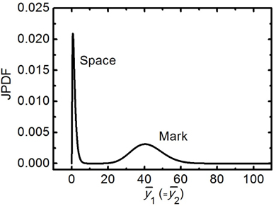
Figure 1 shows two JPDFs evaluated numerically along the = line for A₁ = 40.65 and for A₁ = 0 simultaneously. The former corresponds to the mark and the latter corresponds to the space. The JPDF for the space has been scaled down by the factor of 10 compared with the JPDF for the mark.

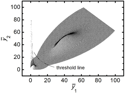
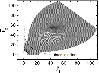
In Fig. 2, we show the foregoing JPDFs in a 3-dimensional way. It has been obtained by adding the JPDFs’ functional values to after multiplying a constant 4×103. Only the points, where at least one of the JPDFs is larger than 10-10, are shown. The JPDF for the space has been scaled down by the factor of 10 here also. Since A₁ = A₂, the JPDFs, including (22), are symmetric with respect to the = = line. Note that f (, ) = 0 when at least one of and is zero. Along the = line, the width of each JPDF increases as increases. In conventional optical receivers, where a threshold voltage is used, we have BER = (2A₁/π)^1/4 exp(− A₁/4)/4 [11], which is 2.2×10^-5. In our case, there is a threshold line as is shown in Fig. 2 where both JPDFs have the same value. The area of each JPDF beyond that line contributes to the BER [5] which is evaluated numerically as 6.8×10^-6. This corresponds to about 0.5 dB enhancement in A₁ compared with the conventional BER of 2.2×10^-5. A₁ and A₂ are actually signal-to-noise ratios [11]. Thus we can have higher system margins using the correlation between the data from the direct-detection optical receiver.

If the two sampling points are T/2 apart with all other parameters fixed, G increases to 0.866. The JPDFs in this case are shown in Fig. 3, which become more circularly symmetric owing to the reduced correlation. The BER is 2.6×10^-7 and the enhancement in A₁ increases to about 1.6 dB. If the two sampling points are 3T/4 apart with all other parameters fixed, G increases to 0.989. The BER is 1.3×10^-8 and the enhancement in A₁ is about 2.4 dB. If the received signal has a different phase between two sampled points, this will decrease H in (18). In this case, our numerical analyses show that the BER decreases as the phase difference increases. Thus our BER values can be reduced introducing the phase change within a bit.

In order to use the threshold line for the decision, we need analog-to-digital converters (ADCs) and digital signal processing (DSP) circuits instead of conventional D-flip-flop type decision. The speed of ADC and DSP circuits has been increased remarkably up to coherent 200 Gb/s per channel during recent years [19]. Realizations of software-defined optical receivers using these devices are now technically feasible and our JPDFs can be used to upgrade their capabilities for IM/DD channels.

We have derived the JPDFs for two voltage data from direct-detection optical receivers in dense WDM systems. We have shown that, with our JPDFs, we can reduce the BER and enhance the receiver sensitivities by 0.5 dB ~ 2.4 dB. Our decision method can be used for software-defined optical receivers supporting both coherent and intensity-modulated channels simultaneously.