Over the last few decades or so, a number of computer-aided alignment estimation methods have been developed. Figoski et al. [1] used the sensitivity table method for alignment of a wide field, three mirror system. Liu et al. [2] found the best set of compensators by calculating the condition number of the sensitivity matrix combination for the target optical system. In the meantime, Kim et al. [3] reported the merit function regression (MFR) method utilizing an optimization algorithm benefitted from multiple wavefront error (WFE) measurements. Generally, they are used to estimate the misalignment state of the selected compensators by using the WFE measurement from multiple fields. On the other hand, Lee et al. [4] proposed Differential Wavefront Sampling (DWS) using the second derivative terms of astigmatism (i.e. diagonal astigmatism, Z5) and the single center field WFE measurement along the optical axis.

While their capability has been well documented however, aforementioned methods tend to neglect the combined effects of practical alignment errors onto the alignment state estimation. These include spatial and temporal variations of environmental conditions in WFE measurement, motion accuracies inherent from the use of alignment tools, etc. In earlier studies, researchers addressed the above effects individually and, to lesser extents, for performance verification of their computer-aided alignment algorithms used in alignment of their target optical system [4-7]. However, the actual alignment runs were made in inadequate accuracy range so that their algorithm performances were not investigated in detail. Furthermore, the effects of field positioning inaccuracy has never been taken into account. Hvisc et al. [8] attempted the singular value decomposition (SVD) analysis to understand the aberration modes when aligning the wide field corrector of the Hobby-Eberly Telescope. Their study resulted in a relationship between the optical component position and their aberration effects, while it did not address the alignment effects from the aforementioned error sources.

There are three important error sources involved in the alignment experiment; field, compensator positioning, and environmental errors. The focus of the interferometer can be placed in an unintended position (i.e. field error) or the movement of compensators can have errors due to the imperfection or low resolution of motion stages (i.e. micrometer positioning error). More critically, the environmental conditions such as air turbulence or vibration during the WFE measurement may affect the resulting interferogram, which causes variations in the Zernike coefficients that are key values to computer-aided alignment (i.e. environmental error). These three errors tend to affect the alignment result in different manners, depending on the algorithm to be used. Therefore, it would be of great usefulness, if the alignment effects of these error sources and their relationships with the alignment state estimation algorithms were analyzed before computer-aided alignment experiment is commenced in optics shops.

In this paper, we first studied the alignment state estimation performances of two algorithms i.e. the sensitivity method and DWS technique under the presence of the above mentioned error sources. We then applied our findings to both simulated and actual computer-aided alignment runs for an infrared optical system (IROS) [9]. Since the two methods use different number of fields and different Zernike coefficients measured, we checked the usefulness of our findings by comparison of their performance results. In Section 2, we describe the error analysis concept and methodology in details. These are followed by the IROS alignment experiment and results as shown in Section 3. Section 4 is concerned with discussion and implications of the analysis results.

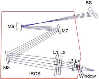
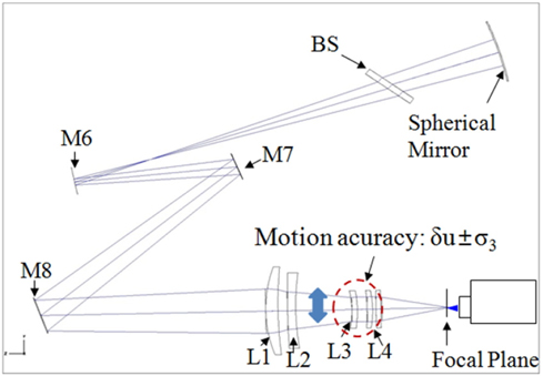
Figure 1 shows the f/2.7 IROS schematic diagram. It consists of three mirrors (M6, M7, and M8) and four lenses (L1, L2, L3, and L4). The front-end telescope, not shown in the figure, delivers the incident light beam onto a dichroic beam splitter (BS) where it is divided into the electro-optical (EO) and infrared (IR) wavelength bands. The EO band (400 nm~900 nm) is focused onto a CCD detector directly after being reflected from BS, while the IR band (3 μm~5 μm) is transmitted through BS and focused onto an IR detector via IROS. The front-end telescope and IROS can be developed separately and assembled together in modular manner. The IROS WFE requirement was to be around 225 nm rms. This was to ensure near-diffraction limited performance at the system level.

The WFE measurement with an interferometer is sensitive to air turbulence and instrument vibration while the measurement data is taken. The influences of environmental disturbances to the estimation of the alignment state were investigated as explained below and in Fig. 2.

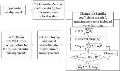
1. Amount of initial misalignment of each compensator is input. They are generally in sub-millimeter scale. This misalignment is to be estimated and then corrected from using the alignment algorithms. 2. The Zernike coefficients of the misaligned optical system wavefront are computed. The sensitivity method uses 5 Zernike coefficients from 5 measurement fields (on-axis and 4 edge diagonal fields); 0°, 45° astigmatism (Z5, Z6), x, y coma (Z7, Z8) and 3rd order spherical aberration (Z9) coefficients. For the DWS method, the field is fixed at the center along the optical axis and the positions of compensators are deliberately perturbed back and forth to obtain two sets of 5 Zernike coefficients (Z5~Z9). 3. The misaligned system rms WFE (W) can be approximated from the root-sum-square (RSS) of the measured Zernike coefficients (Z5~Z9) obtained from all fields in the sensitivity method and all positions in the DWS method. 4. The environmental error range (σ1) is then set. It is experimentally determined from using the standard deviation (SD) of repeatable WFE measurement in actual alignment practice. 5. The random numbers (αi) are generated according to a normal distribution with zero average and SD of σ1. These numbers are added to each Zernike coefficient to make an erroneous Zernike coefficient (Zi+αi). This is to simulate the random effects of environmental variation such as instrument vibration or air turbulence. We then calculate the RSS of the erroneous Zernike coefficients (WE). 6. If the difference between W and WE is larger than σ1, other random numbers are generated to produce a new set of erroneous Zernike coefficients in step 5. This process is repeated until the criterion is met as in step 6 in Fig. 2. 7. Employing alignment algorithms, the amounts of current misalignments for each compensator is derived. The final rms WFE is then calculated after compensating for the estimated initial misalignments. 8. The process step 5~7 are repeated 100 times to obtain the averaged rms WFE and its standard deviation.

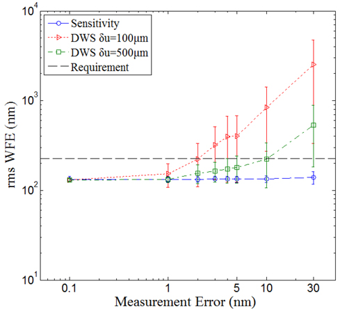
Figure 3 shows the analysis results at the four edge fields. The initial misalignments of compensators were set to 0.5 mm. The environmental error used varies from 0.1 nm to 30 nm rms. 0.1 nm was used to simulate the best measurement accuracy of a commercial interferometer, while 30 nm was to represent the measurement under the harsh environmental conditions. The total 100 iterative computations were carried out for each environmental error input.

For the DWS method, two different perturbations (δu) of 100 μm and 500 μm for each compensator were used. Initially, the 500 μm perturbation case was analyzed to set the reference response, even though it generated WFE too large to be measured with a commercial Fizeau type interferometer. Figure 3 shows remarkably stable results within the requirement from the sensitivity method, while the DWS method tends to increase rms WFE significantly beyond the requirement as the measurement error increases. We believe that the higher robustness of the sensitivity method than for DWS comes from the average-out effects of random environmental errors by using more parameters; the sensitivity method utilizes 25 parameters (i.e. 5 Zernike coefficients at 5 different fields), whereas there are only 10 parameters used for DWS method (i.e. 1 Zernike coefficients, which is Z5, at 10 different positions - 5 compensators per deliberate perturbation at single field).

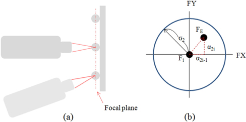
As the sensitivity method uses multiple field WFE measurements while DWS uses the single field, the measurement field error can be further amplified for the sensitivity method than for DWS. Figure 4(a) shows the concept of multiple field WFE measurement. A reference iron ball is placed at the measurement focal plane and the distance variation between the interferometer and the focal plane is continuously adjusted. In this arrangement, the field position error in the optical axis (Z) direction plays an insignificant role during the measurement. We can then consider x and y axis position errors as in Fig. 4(b). FX and FY are field directions along x and y axis. F_i is the ideal position, F_E the actual position with the error included, σ₂ the maximum field error in radius and α (α_2i-1 and α_2i means odd and even numbers) the error at each axis. After setting up the interferometer position, the iron ball is removed and the IROS WFE is measured. In this manner, we can measure and analyze the field error for the sensitivity method.

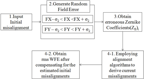
For analysis of field error in the sensitivity method, the following steps were applied as shown in Fig. 5.

1. The analysis step 1 is as same as in the environmental error case already mentioned. The amount of initial misalignment is given to each compensator and it needs to be computed and corrected. 2. The total 10 random field errors with given range (σ2) are generated and added to each normalized field to represent field error; ((0±α1, 0±α2), (1±α3, 1±α4), (1±α5, -1±α6), (-1±α7, 1±α8), (-1±α9, -1±α10)). The z-axis error is not considered, as it is calibrated with the iron ball at the focal plane. 3. We obtain 0° and 45° astigmatism (Z5, Z6), x and y coma (Z7, Z8) and 3rd order spherical aberration (Z9) coefficients from 5 measurement fields (on-axis and 4 edge diagonal fields) inclusive of the field position errors. 4. The alignment algorithm is then used to estimate the current misalignment for each compensator. The final rms WFE is then obtained after compensating for the estimated current misalignments. 5. The process steps from 2 to 4 are repeated to derive the average rms WFE and its SD.

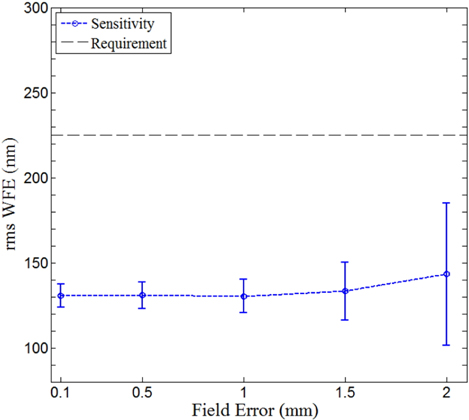
Figure 6 shows the analysis results, showing the mean WFE and SD bar from 100 iterative simulations at 5 fields (4 edge fields and on-axis field). The aligned WFE is located within the requirement for all fields over the field error range from 100 microns to 2 mm. This implies that the sensitivity method is very well immune to the field position error in wavefront measurement.

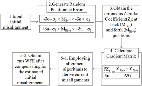
For the case of the sensitivity method, the positioning error does not occur, as the compensators are stationary during the WFE measurement. On the other hand, the positioning error of compensator stages affects the alignment estimation performance of the DWS method as it requires for the deliberate perturbation of compensator location along the mount axis, in order to obtain the gradient of 0° astigmatism (Z5). The concept of the positioning error model is depicted in Fig. 7. Here the decenter of L3 and L4 in X and Y, and their lateral shift along the light path are of main interests to the analysis model. Their intended motion (δu) and its unexpected error (σ₃) taking place during the alignment action are drawn in Fig 7.

The model analysis steps follow the procedure listed below and as shown in Fig. 8.

1. The analysis step 1 is as same as in the environmental error case already mentioned. The amount of initial misalignment is given to each compensator and it needs to be computed and corrected. 2. The random positioning error within the range (σ3) is generated and input to the deliberately perturbation of the compensator back (-δu) and forth (+δu). This is to represent the position accuracy of the compensator mount in alignment action. 3. We then obtain the erroneous 0° astigmatism (Z5) coefficients from the on-axis field at back (ME(-)) and forth (ME(+)) positions. 4. The gradients of Z5 are computed for each compensator movement. Z5(+) is obtained from the forward (ME(+)) perturbation positions and Z5(-) from backward (ME(-)) perturbation positions. For the calculation, the deliberate perturbation range is fixed to 2δu. 5. The alignment algorithm is used to estimate the current misalignments of each compensator. The final rms WFE is then obtained after compensating for the estimated current misalignments. 6. The process steps from 2 to 5 are repeated to obtain the average final rms WFE and its SD.

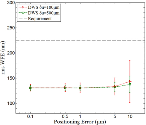
Figure 9 shows the model analysis results for two perturbation cases of 100 μm and 500 μm. Each point in the graph is the mean WFE and SD bar derived from 100 iterative computations only at the on-axis field. The resulting rms WFE remains stationary over the positioning error range from 0.1 micron to about 5 microns and it increases marginally between 5 microns to 10 microns in range. Nevertheless, the trend is clear that it remains well below the requirement. This implies that the DWS method is practically insensitive to the micrometer positioning error when aligning IROS. In summary, we gathered convincing evidence that, for the actual IROS alignment run, we do not need to be concerned about the field error if the sensitivity method was to be used and the positioning error if the DWS method was to be applied.

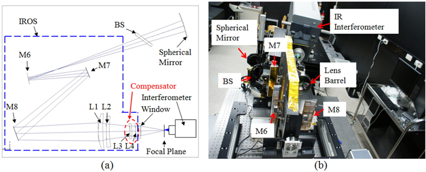
Trial alignment runs were made for IROS with the sensitivity and DWS methods. Figure 10(a) shows the schematic diagram of the alignment set-up and Fig. 10(b) is a photograph of the actual experiment configuration. The IR interferometer sends a spherical wave of f/2.5 to the IROS focal plane. It passes through the transparent window and lens group from L4 to L1. The IR beam is reflected from M8 toward M6. As explained in Section 1, in order to simulate the front-end optics, a parallel plate and a spherical mirror of 100 mm in diameter and of 529 mm in curvature of radius are added; the parallel plate acts as a BS of front-end optics and a spherical mirror reflects the spherical wave generated by IROS back to the interferometer.

A Fizeau type IR interferometer operating at 3.39 μm in the wavelength of the He-Ne laser was used for the wavefront measurement. As expressed already, the initial sensitivity analysis defined the compensators for alignment as L3 decenter (x,y), L4 decenter (x,y) and L4 despace (see Figure 1) [10]. The tolerances were set to 0.05 mm for all the compensators. The main compensator L3 and L4 were mounted on a commercial two-axis linear stage with 10 μm in micrometer resolution. The IROS optical design defines 124 nm in rms WFE for the center field and 225 nm for the whole field target performance. The IROS is designed to operate 4200 nm in wavelength and, with the above mentioned WFE target, it is expected to show a near diffraction limited performance.

100 WFE measurements were made at each field and the resulting WFE data were averaged to understand the environmental error influence to the system wavefront. The measurements were made over all 5 fields and the results show 2 nm rms in SD. This leads to, according to Fig. 3, the IROS alignment state influence of 132 nm would be arising from the sensitivity method and of 223 nm with 115 nm in SD from the DWS method under the deliberate perturbation of 100 μm. It would be further aggravated if we take the surface error of 30 nm rms in average for total 14 surfaces into consideration. In this case, the alignment state would worsen to 174 nm in RSS for the sensitivity method and 249 nm for the DWS method. Therefore, it was predicted that the application of sensitivity method to the IROS alignment would satisfy 225 nm in the target WFE requirement, while the DWS method would not produce such successful results.

Having understood the aforementioned environmental influences to the alignment state estimation, we measured rms WFE at the center and 4 edge fields before the commencement of the IROS fine alignment. As shown in Fig. 11, the results vary from 966 nm to 1004 nm over 4 edge fields and 216 nm at the center. These are clearly beyond the requirement of 225 nm rms. From the measurement data, the Zernike coefficient set was extracted for the sensitivity method while, for the DWS method, Z5 (0 degree astigmatism) was derived at the center field with 100 μm of perturbation in both directions of compensators. This amount of perturbation was nearly the maximum limit of the practical WFE measurement with a commercial Fizeau type IR interferometer for IROS.

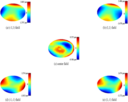
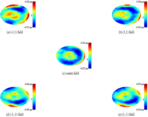
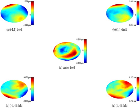
Figure 12 shows the WFE measurement results after the alignment run using the sensitivity method. The resulting WFE distribution varies from 157 nm to 188 nm for the off-axis fields (168 nm in average) and they are quite close to 174 nm that is the theoretical expectation. The alignment results with DWS method are shown in Fig. 13, ranging from 208 nm to 359 nm for the off-axis fields (262 nm in average) and 116 nm for the on-axis center field. These values also fall close to our expectation, 249 nm, even though the application of DWS method to the IROS alignment would produce less successful results across all fields. Specially, the WFEs of 359 nm at (-1,1) field and 275 nm at (1,1) field do not meet the requirement of 225 nm, whereas the other field shows marginally close to satisfaction. In general, the above mentioned experimental results demonstrate that the prior analysis of practical error sources in alignment can be an effective tool for choosing the proper alignment algorithm and for efficient alignment process.

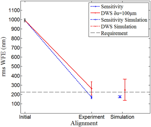
Figure 14 shows both predicted and experimented rms WFE data of IROA just after the initial integration and after the fine alignment. The measured environmental wavefront error of 2 nm rms and the averaged surface figure error of 30 nm rms WFE for 14 surfaces in total were added to form the data shown in the figure. The initial wavefront error is the averaged value of all the wavefront error data appeared in Fig. 11, while those of “Experiment” and “Simulation” are from the data depicted in Fig. 12, Fig. 13. and Fig. 3.

First, we note that the simulated average rms WFE is 174 nm and it is very close to 168 nm from the experiment. And their field imbalances are 10 nm in simulation and 14 nm from the measurement respectively. On the other hand, the average rms WFE from the DWS simulation turns out to be 249 nm but 262 nm in experiment. Their field imbalances are 112 nm in simulation and 71 nm in experiment respectively. The close proximity of predicted and experimental WFE tells us that all the influences from those practical alignment error sources have been well accounted for in both simulation and experiment analysis of the alignment state. We also note that the field error effects to the sensitivity method performance and the positioning error effects to the DWS method performance are negligible as predicted in section 2. However, the error analysis can suggest how the DWS method can be better used; for example, if the environmental error can be reduced to less than 1 nm rms or the optical system is capable of dealing with 400 μm or larger perturbation, then the IROS can be aligned to within the requirement by using the DWS method. To those extents, the error analysis method presented in this study is an efficient tool to increase the WFE estimation performance of the alignment algorithm and therefore the process efficiency of actual alignment run.

While environmental, measurement field and micrometer positioning errors play important roles in decreasing the process efficiency of the computer-aided alignment, earlier studies [1-7] gave less academic attention to these very subjects. On the contrary, this study addresses detailed modeling and analysis of such error sources influencing the alignment estimation performance for actual alignment run. The analysis results show that the environmental error plays the most significant role in degrading the alignment process efficiency, whereas the influences from the field and positioning error can be negligible depending on the choice of alignment algorithm used.

We applied these findings to the application of sensitivity and DWS algorithms for alignment of IROS both in simulation and in experiment. The results show that the sensitivity method gave the aligned WFE thus satisfying the requirement, while the DWS method was less successful. This demonstrates that, with prior error model analysis of the target optical system using the alignment algorithms, a proper alignment method can be selected depending on what plays the role of the primary alignment error source, even before the actual alignment run commences. We believe that the work and findings presented in this study would contribute greatly to the increasing process efficiency for actual alignment run during the final integration and testing phase for high performance optical systems.