Northern wetlands are important ecosystems; the arctic tundra covers approximately 5% of global land area and contains approximately 12–14% of the world's total pool of soil organic carbon (Post et al. 1982). Furthermore, the arctic tundra is one of the most sensitive ecosystems in response to climate change because of feedback effects, such as the transition from snow and ice to water and land. Bekryaev et al. (2010) determined that both land and sea-surface temperature have increased rapidly in most parts of the Arctic, with rates up to 1.35ºC per decade during 1998–2008, and sea ice has melted approximately 10% per decade between 1979 and 2007 (Comiso et al. 2008). These environmental changes are having effects on the Arctic tundra vegetation, and a detailed analysis of these effects is required.
Arctic vegetation patterns are determined by differences in climate, topography, and soils (Britton 1967, Peterson and Billings 1980), and several studies of vegetation patterns have been carried out on scales of several meters to a few kilometers. Most past studies described linear vegetation patterns depending on topography by using transect-sampling methods. We used a gridsampling method and applied geostatistics to analyze spatial variability and patterns of vegetation within twodimensional space. Geostatistical methods can describe spatial variability in vegetation using semivariograms and correlograms, and can further predict vegetation distribution of unsampled areas using kriging (Goovaerts 1999). Recent studies on vegetation patterns in response to climate change have mainly focused on satellite imagery using the normalized difference vegetation index (NDVI), an important tool for description at the regional scale; but until now, it was not possible to determine each species at the grassland by using the NDVI. In the present study, we analyzed the distributional patterns of each plant species and their associations in the arctic tundra ecosystem.
Plant distribution was estimated by simple inverse distance (Bregt et al. 1992), autocorrelation (Nordbo et al. 1994), or kriging (Heisel et al. 1996). These methods take into account spatial dependence, but only kriging ensures that the estimation is unbiased and has minimum variance (Cressie 1993). Geostatistical methods such as semivariograms, correlograms, and kriging have been applied to estimate vegetation distribution (Heisel et al. 1999, Rew and Cousens 2001).
The purposes of this study are as follow: (1) to present spatial distributional characteristics of 8 tundra plants that are dominant species in council, Alaska; and (2) to assess the spatial association among tundra plant species in a 10,000 m2 area.
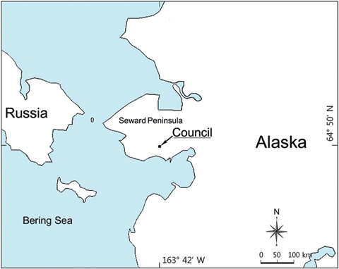
The study was conducted in Council, Alaska (64º50′ 38.6″ N, 163º42′39.6″ W), in an area where representative arctic tundra vegetation was found (Fig. 1). Alaska tundra was classified into 8 broad vegetation types (Johnson and Vogel 1966). More specifically, our study site can be defined by
A grid-sampling method was applied to determine the spatial variability of Alaska tundra vegetation. In July 2010, we placed 66 quadrats at the intersects of a 20 m × 10 m grid within the 100 m × 100 m plot for measuring vegetation coverage. The abundance of vegetation was measured as the coverage within a 50 cm × 50 cm quadrat. Coverage is thought to be an ecologically important single parameter of a species in relation to its community because it is an estimate of how much a plant dominates an ecosystem (Lindsey 1956, Daubenmire 1959). Vegetation coverage was measured in the field, and we took a photograph of each quadrat and checked the coverage in the laboratory using image-analysis software (Image J 1.34 s; Wayne Rasban, National Institutes of Health, USA).
The coverage of 8 species was analyzed using classic statistical descriptors such as mean, coefficient of variance, skewness, kurtosis, and Pearson’s correlation coefficient. Diverse transformations were performed to obtain a nearly normal distribution, because geostatistical analyses are sensitive to highly skewed distribution (Jongman et al. 1995). The importance value of each species was calculated based on the relative coverage and relative frequency.
Spatial autocorrelation of species was calculated with a permutation test for Moran’s

where
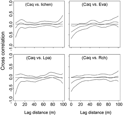
The cross-correlogram was applied to figure out the spatial correlation existing between two species. We used the spline cross-correlogram, which is an adaptation of the nonparametric covariance function (Bjørnstad et al. 1999, Bjørnstad and Falck 2001) that provides a 95% confidence envelope for the function with a bootstrap algorithm. The nonparametric covariance function is calculated as follows:
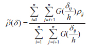
where
Interpolated maps were computed using the block kriging method, which involves estimating values for areas within the unit. Block kriging is more appropriate than punctual kriging methods because average values are more meaningful than single point values (Burgess and Webster 1980). To define the degree of autocorrelation among the measured data points, the semivariance statistic γ(
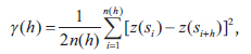
where
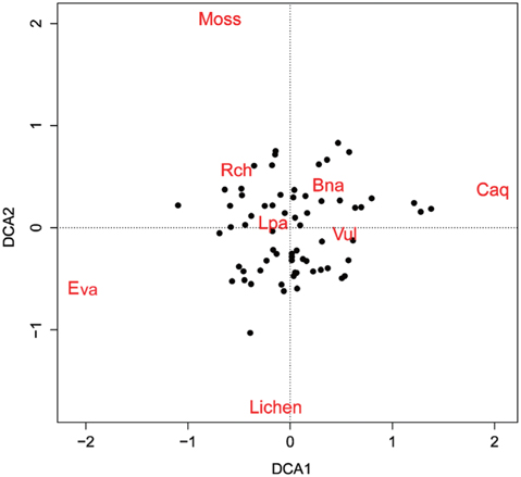
To analyze compositional differences among the plant communities of the 66 surveyed quadrats, Detrended Correspondence Analysis (DCA) ordination techniques were applied using the “vegan” package ver. 2.0-7 of the R program (Oksanen et al. 2007). DCA was developed to overcome the distortions inherent in correspondence analysis ordination, and performs better with simulated data than do correspondence analyses or reciprocal averaging ordinations (Hill and Gauch Jr 1980). The Bray–Curtis coefficient was used for a distance measure because it is known as one of the most robust measures (Faith et al. 1987).
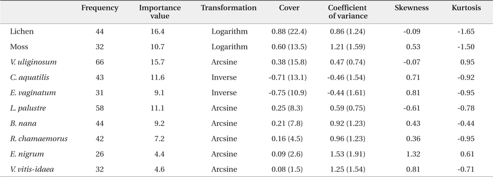
A total of 12 species and 7 families of vascular plants were identified in the study site. The descriptive statistics for the 10 dominant plants are shown in Table 1. The most frequently found vascular plant species were

Descriptive statistics of percent cover of the 10 dominant plant species and vegetation types in arctic tundra in Council, Alaska. The figures in the brackets are untransformed data values
In our study area, the most important vegetation was lichen. Moss had an importance value approximately 35% lower than that of lichen. V. uliginosum had the highest importance value among 8 vascular plant species, followed by
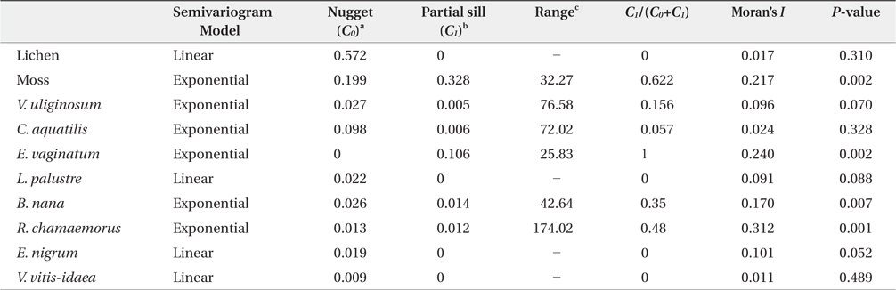
Parameters of the semivariogram model and Moran’s I statistics for the 10 dominant vegetations in arctic tundra, Council
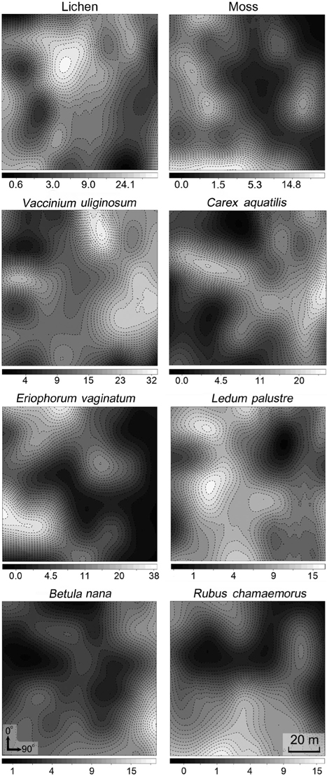
The spatial patterns of vegetation at the study plot are presented in Fig. 3. A visual assessment reveals the distribution patterns and spatial correlation among vegetation.
The four DCA axes had eigenvalues of 0.20, 0.16, 0.13, and 0.11, and the first two axes were used to generate the scatter plot shown in Fig. 5.
Understanding vegetation distribution patterns may be an important step for recognition of arctic tundra ecosystems and their response to climate change. Geostatistics can be a suitable method for understanding spatial variability and interpolation of vegetation distribution maps (Heisel et al. 1999, Jurado-Expόsito et al. 2004). In the arctic tundra, several studies have applied geostatistical methods using NDVI datasets for recognition of vegetation patterns at the broad scale (Allen et al. 2004, Spadavecchia et al. 2008), but few studies have applied geostatistical methods to shrubs or herbaceous plants at the micro-habitat scale.
Viereck et al (1992) classified Alaska tundra according to a five-level criterion. Our study site, Council, Alaska, may belong to tussock tundra because tussock (
In our study site, 5 out of 12 species were included in family Ericaceae, which is common in nutrient-poor sites such as heathland and arctic tundra. The soil at our site was also barren in terms of nitrogen content. The presence of mycorrhizae in Ericaceae plants may help to enhance nitrogen absorption (Strandberg and Johansson 1999), which may be main reason why Ericaceae flourish in our study site, arctic tundra. In addition, the most dominant vascular species in our study site was
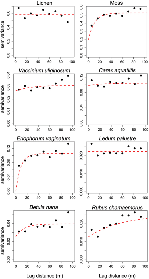
Geostatistics results showed diverse distributional pattern of tundra vegetation. Semivariance ideally increases with lag distance, and the distance where the model first flattens out is called as the range; sill is semivarance value at the range. Samples separated by distance closer than the range are related spatially. Whereas, those sperated by distances greater than the range are not spatially related (Cambardella et al. 1994). Theoretically, the semivariance should be zero at zero separation distance. However, the semivariance usually does not have zero. This is called the nugget effect. The nugget effect is often caused by spatial sources of variation at distances smaller than the sampling interval (Zhao et al. 2009). Our results showed that many species had relatively high nugget values, except for moss and
Spatial partitioning of resources and interactions with other species can determine the distribution of species (Chapin III and Shaver 1985). On the contrary, spatial distribution of well-known species can provide clues about limiting environmental factors or competition with other species. Interpolation maps, cross-correlograms, and DCA biplot revealed the spatial specificity of
In summary, our study site is representative tussock tundra comprising a small waterway.