검색 전체 메뉴
PDF
맨 위로
OA 학술지
Statistical Properties of Geomagnetic Activity Indices and Solar Wind Parameters
  • 비영리 CC BY-NC
  • 비영리 CC BY-NC
ABSTRACT
Statistical Properties of Geomagnetic Activity Indices and Solar Wind Parameters
KEYWORD
Solar wind , IMF , geomagnetic index , data analysis
  • 1. INTRODUCTION

    One of hot issues of solar-terrestrial physics is the prediction of intensity of geomagnetic storms and moments when they are occurring, which is a main problem of a subject now known as space weather forecast. Geomagnetic storms are phenomena that last a few days during which the geomagnetic field experiences rapid variations seriously affecting human activities (e.g., Eroshenko et al. 2010). The magnetic variations are a proxy for disturbances in the plasma populations and electric current systems present in the terrestrial magnetosphere. They are, however, responsible for at most around 1% of the total magnetic field that can be measured at the Earth’s surface. For instance, even in the severe cases they are between 400 and 700 nT against 40000 nT in normal regions. The primary energy source of the geomagnetic storm is the Sun which transfers energy to the Earth’s magnetosphere by means of solar wind. Energy from solar wind is injected into the Earth’s magnetosphere mostly in a case when interplanetary magnetic field (IMF) has a significant southward component (Cane et al. 2000). This magnetic field orientation allows magnetic reconnection and energy transfer from solar wind to the Earth’s magnetosphere. When accumulated energy reaches a certain level, any small disturbance outside or inside Earth’s magnetosphere can result in violent release of this energy as global reorganization of electric current systems of Earth’s magnetosphere and heating/acceleration of plasma. Although the geomagnetic storm has been attributed to solar phenomena for decades, the exact solar sources and their characteristics have not been well defined (e.g., Gonzalez & Tsurutani 1987, Wang et al. 2002, Cane & Richardson 2003, Correia & de Souza 2005, Yermolaev et al. 2007).

    Temporal variations of such key parameters have been extensively investigated. Firstly, the 11-year solar cycle and associated variabilities have been studied in the last decades to understand actual mechanisms and processes for the observed geomagnetic storms. Periodicities of ~ 11 years, ~ 5.3 years, ~ 3.5 years, ~ 1.9 years and even shorter ones are found being meaningful using harmonic analysis of IMF parameters and/or geomagnetic activity indices (Kane 1997, Ahluwalia 2000, Clúa de Gonzalez et al. 2001, Kane 2005, de Artigas et al. 2006, Oh & Chang 2012, Cho et al. 2014). The solar cycle dependence of geomagnetic storm occurrence has been further studied. Geomagnetic storms are more likely to arise near the sunspot maximum and in the descending phase of the solar cycle as well (Gonzalez et al. 2007, Echer et al. 2008). Secondly, the annual geomagnetic activity distribution is frequently being reported, which is characterized with maxima around the equinoxes and minima near the solstices. The cause of this seasonal variation may be attributed to one or more of the three models known respectively as the equinoctial hypothesis, the axial hypothesis and Russell-McPherron mechanisms (Russell & McPherron 1973, Clúa de Gonzalez et al. 1993, Clúa de Gonzalez et al. 2002). Thirdly, a correlation between distributions and the corresponding geomagnetic storm intensities has been also found, which is actually regarded as a basis of solar-terrestrial connection. This finding could serve as a probabilistic storm forecasting method (e.g., Crooker & Gringauz 1993).

    Yet another useful technique for solving problems in the subject of space weather is the calculation of frequency distributions of events, that is, occurrence rate, based on observations, whose form can be dN(x) = F(x)dx where dN(x) is the number of events for a given parameter x of interest between x and x + dx, and F(x) is a frequency distribution (e.g., Dias & Papa 2010, Riley 2012). As efforts in deriving the occurrence probability of a geomagnetic storm event of a given intensity the distribution of solar wind parameters and geomagnetic indices has been explored. Statistical studies show that the Gaussian approximation well suits for some parameters, while for others the lognormal law seems preferred (Tsurutani et al. 1990, Bristow 2008, Veselovsky et al. 2010, Yermolaev et al. 2013). Echer et al. (2011) have also reported that geomagnetic storm peak intensity distribution can be described by an exponential form. This exponential distribution indicates that intense events have a much lower probability of occurrence than weaker storms. In this study we carry out detailed statistical analysis of solar wind parameters and geomagnetic indices. The study has been undertaken with two primary goals. The first is to examine the distribution of such key parameters relating the geomagnetic storm, which may subsequently lead us to the occurrence rate of the geomagnetic storm. It may well provide a very important clue in presenting a probabilistic model of geomagnetic storms and possible physical causes. The second is to examine the dependence of the distribution on the solar cycle and annual variations. Likewise for the first aim, outcomes may provide the dependence of the occurrence probability of geomagnetic storms. This paper is organized as follows. We begin with brief descriptions of data analyzed for the present paper and a way of analysis in Section 2. We present and discuss results of analysis in Section 3. Finally, we summarize and conclude in Section 4.

    2. DATA AND METHOD OF ANALYSIS

    For the present analysis, firstly, we have used the mean daily speed of solar wind and the number density of protons (np in # cm-3) in solar wind during the period from February in 1999 to January in 2013. They are measured by the Solar Wind Electron, Proton, and Alpha Monitor (SWEPAM) on the Advanced Composition Explorer (ACE) spacecraft. Both data sets can be obtained from the ACE Science Center website1. Secondly, we have used the IMF data observed during the same period by the Magnetic Field Experiment (MAG) on the ACE spacecraft. We adopt field values in the Geocentric Solar Magnetospheric (GSM) coordinate system, where the X-axis is parallel to the Earth-Sun line and Z-axis is the projection of dipole axis on the YZ plane of the Geocentric Solar Ecliptic (GSE) coordinate system, the Z-axis of the GSE coordinate system being the ecliptic north pole. Data have been taken from the ACE Science Center website. Thirdly, we have used the Dst index and the AE index observed during the period from February in 1999 to January in 2013. The Dst index describing the development of global large-scale geomagnetic storms is connected to the geomagnetic field near the equator and to the condition of the ring current. The Dst index is maintained at National Geophysical Data Center (NGDC)2 and is available via FTP3. The AE index, on the other hand, is designed to provide a global measure of auroral zone magnetic activity produced by enhanced Ionospheric currents. The AE index can also be downloaded via FTP4 of NGDC sites.

    The present analysis is carried out using the superimposed epoch method for 10 parameters in total as listed in the next section (Kim & Chang 2014). To apply the technique for a selected parameter, we first chop the entire data-string of time series into several substrings with an appropriate length. Then we superimpose substrings and in turn average values of the parameter of interest for a given epoch, respectively. We end up with one single shortened data-string after this step of process. For instance, in comparing statistical properties at the solar maximum and minimum periods, we have 365 day long substrings. Or, in examining the dependence of the distribution on the annual variation we have 6 month long substrings because of 2 equinoxes and 2 solstices, respectively. Having done that, in order to construct the distribution function we need to count the number of values of the parameter of interest in each bin, resulting in a histogram. Note that the histogram is normalized such that the total area is equal to the unity. Finally, we fit the Gaussian function to the histogram by independently adjusting 3 parameters (amplitude, mean value, width) assuming a normal distribution of errors. We repeat the whole procedure for sub-samples into which the parent data sample is divided by the predetermined criteria. Details of each step in the procedure are slightly subject to the parameter we study. For instance, we have arbitrarily chosen the bin size depending on the parameter under examination. However, the conclusion we draw is insensitive to the details.

    3. RESULTS AND DISCUSSIONS

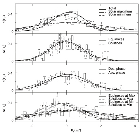
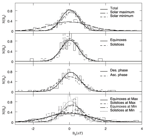
    The analysis introduced in the previous section is carried out for the bulk speed of solar wind, he proton density in solar wind, magnitudes of the total IMF |B| and of its three components in the GSM coordinate system, BX, BY, BZ, the approximate Kan-Lee merging electric field BV (Kan & Lee 1979), the solar wind driving function associated with the solar wind energy flux BV2 (Akasofu 1981), the AE index, and the Dst index. The Kan-Lee merging electric field BVYZ or the eastward component of the interplanetary electric field VXBZ, the solar wind driving function BV2 are all known to give an excellent correlation with the geomagnetic index and effective in producing large-scale geomagnetic disturbances (Crooker & Gringauz 1993).

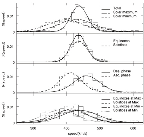
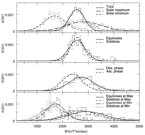
    In Fig. 1, we show histograms of the speed of solar wind and their best fits obtained using the Gaussian function. In the top panel, we show histograms resulting from the whole data set of 14 year long duration and two sub-samples corresponding to the durations including the solar maximum (1999.02-2002.01) and the solar minimum (2008.02-2011.01), respectively. Solid, longdashed and short-dashed curves indicate the total data set, the subsets denoting the solar maximum, and the solar minimum, respectively. Thick curves represent the best fits of the Gaussian function to each histogram. Same line types represent same data sets. The Gaussian function is apparently a good approximation of the histograms. It is not a surprising result in the sense that according to the central limit theorem of the probability theory the Gaussian distribution originates as a result of summation of independent random quantities. According to the Gaussian fit, the mean value resulting from the subset of the solar maximum is greater than that of the solar minimum. This is not unexpected, either, since more frequent solar activities are expected in the solar maximum period (Gonzalez et al. 2007, Echer et al. 2008). It should be noted, however, that the full-width-at-half-maximum (FWHM) resulting from the subset of the solar maximum is larger than that of the solar minimum. Hence, we conclude that intense solar wind may be expected due to not only the large mean value but also the nature of the broad distribution. This fact also indicates that during the solar maximum period one may expect much slower solar wind with respect to its mean value somewhat equally with much faster solar wind. Fitting parameters are listed in Table 1.

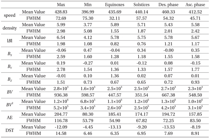
    [Table 1.] Gaussian parameters obtained with fittings to histograms.

    label

    Gaussian parameters obtained with fittings to histograms.

    In the second panel, we show histograms resulting from the two sub-samples corresponding to the durations including the two equinoxes (6 months of the year around the vernal and autumnal equinoxes) and the two solstices (6 months of the year around the summer and winter solstices), respectively. Solid and short-dashed curves indicate the subsets denoting the equinoxes and the solstices, respectively. Thick curves represent the best fits of the Gaussian function to each histogram. Same line types represent same data sets. Unlike other criteria in subgrouping the data sets a result here is somewhat different from what one might have expected. In other words, one is likely to expect the larger mean value and the FWHM for the sub-sample of the equinoxes than the solstices, since the annual geomagnetic activity distribution with maxima around the equinoxes has been reported in earlier reports (e.g., Clúa de Gonzalez et al. 2002). As a result of our analysis, as shown in the last panel, this effect is emanated more clearly when the data sets are further divided in terms of the solar maximum/minimum. Fitting parameters are listed in Table 1.

    In the third panel, we show histograms resulting from the two sub-samples corresponding to the durations including the ascending phase of the solar cycle (1999.02-2002.01, 2009.02-2013.01) and the descending phase of the solar cycle (2002.02-2009.01), respectively. Solid and shortdashed curves indicate the subsets denoting the descending phase and the ascending phase, respectively. Thick curves represent the best fits of the Gaussian function to each histogram. Same line types represent same data sets. In this case, as seen in the solar maximum and minimum case, we find that the mean value and the FWHM for the sub-sample corresponding to the descending phase of the solar cycle are greater than the ascending phase. This finding appears to agree with earlier studies reporting that a physical condition of IMF is more chaotic in the descending phase than in the ascending phase of the solar cycle (Gonzalez et al. 2007, Echer et al. 2008). Fitting parameters are listed in Table 1.

    In the last panel, we show histograms resulting from the four sub-samples corresponding to the durations including the two equinoxes (6 months of the year around the equinoxes) in the solar maximum (1999.02-2002.01) and in the solar minimum (2008.02-2011.01), and the two solstices (6 months of the year around the summer and winter solstices) in the solar maximum (1999.02-2002.01) and in the solar minimum (2008.02-2011.01), respectively. Solid, shortdashed, long-dashed and dotted curves indicate the subsets denoting the equinoxes in the solar maximum, the solstices in the solar maximum, the equinoxes in the solar minimum and the solstices in the solar minimum, respectively. Thick curves represent the best fits of the Gaussian function to each histogram. Same line types represent same data sets. Basically, what we see is what we may expect from plots shown in the first and the second panels. It apparently shows more clearly than the second panel characteristic features expected from the fact that the annual geomagnetic activity distribution has a maximum around the equinoxes. Fitting parameters are listed in Table 1.

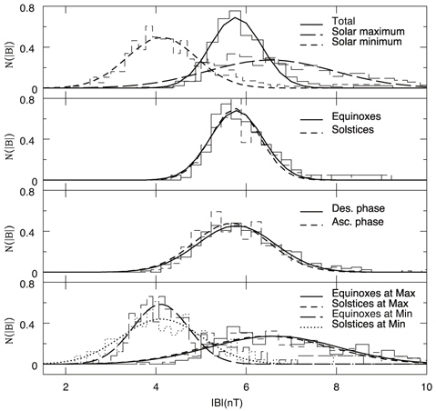
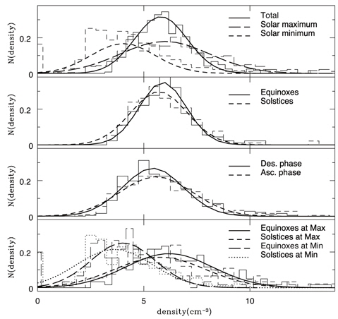
    In Fig. 2, we show similar plots resulting from the proton density in solar wind. In this particular example, the distributions of the proton density seem comparable each other both in the descending/ascending phases of the solar cycle and in the equinoxes/solstices. On the other hand, they are distinct in the solar maximum/minimum according to the first panels. Fitting parameters are listed in Table 1. In Fig. 3, we show similar plots resulting from the total magnitude of the IMF |B|. The distributions of the IMF |B| are almost indistinguishable in the descending/ascending phases of the solar cycle and in the equinoxes/solstices. Notably, however, they show a significant difference in the solar maximum/minimum according to the first panels. Fitting parameters are listed in Table 1. In Figs. 4-6, we show similar plots resulting from the magnitudes in its three components of the GSM coordinate system of the IMF, respectively. The most crucial factor in characterizing the distribution seems whether data sets include the period around the solar maximum or the solar minimum as seen in elsewhere. The phase in the 11-year solar cycle and annual variations appears less effective compared with the level of solar activity. Fitting parameters are listed in Table 1.

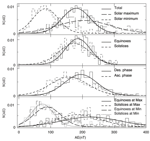
    In Figs. 7 and 8, we show similar plots resulting from the approximate Kan-Lee merging electric field BV and the solar wind driving function BV2, respectively. The distributions of BV and BV2 are all dependent on the solar maximum/ minimum, the descending/ascending phases of the solar cycle and the equinoxes/solstices. Nonetheless, the level of solar activity appears the most crucial among these. Fitting parameters are listed in Table 1. In Figs. 9 and 10, we show similar plots resulting from the AE index and the Dst index, respectively. As in cases of BV and BV2, the distributions of the AE index and the Dst index are all subject to the solar maximum/minimum, the descending/ascending phases of the solar cycle and the equinoxes/solstices. The level of solar activity appears again the most critical among criteria in sub-grouping the data sets. Fitting parameters are listed in Table 1.

    4. SUMMARY AND CONCLUSION

    Geomagnetic storms affect human activities in the modern age. Thus, the prediction of geomagnetic storms is becoming a more and more important and practical problem. An effective approach could be dealing with it as a probabilistic geomagnetic storm forecasting problem. To do so, one requires the occurrence probability function of a geomagnetic storm event for a given intensity. As a contribution to this line of efforts, we carry out detailed statistical analysis of solar wind parameters and geomagnetic indices in this study. Hoping to help in presenting a probabilistic model of geomagnetic storms, we have also examined the dependence of the distribution on the solar cycle and annual variations. The distribution of geomagnetic storms throughout the solar cycle and during the calendar year is a very important topic in space weather.

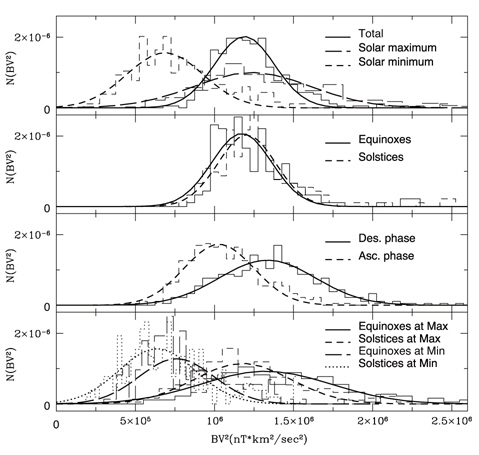
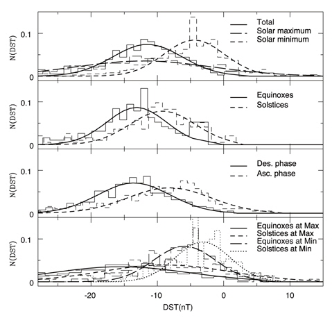
    What we have found are as follows: (1) The distribution of parameters obtained via the superimposed epoch method follows the Gaussian distribution. It can be understood according to the central limit theorem of the probability theory. (2) The distribution of all the examined parameters is most sensitively dependent on the level of solar activity. When solar activity is at its maximum the mean value of the distribution is shifted to the direction indicating the intense environment. Furthermore, based on our analysis the width of the distribution becomes wider at its maximum than at its minimum so that more extreme case can be expected. (3) In general, the distribution of heliospheric parameters, such as, solar wind parameters and magnitudes of the IMF, is less sensitive to the phase of the solar cycle and annual variations. That is, the distributions seem comparable regardless of the descending/ascending phases of the solar cycle and in the equinoxes/solstices. (4) The distribution of the eastward component of the interplanetary electric field BV and the solar wind driving function BV2, however, appears to be all dependent on the solar maximum/minimum, the descending/ascending phases of the solar cycle and the equinoxes/solstices. Even in this case, the solar maximum/minimum is the most critical factor. (5) The distribution of the AE index and the Dst index shares statistical features closely with BV and BV2 compared with other heliospheric parameters. They are wider during periods of the solar maximum, the declining phase of the solar cycle and the equinoxes. In this sense, BV and BV2 are more robust proxies of the geomagnetic storm. As a result of our findings we conclude that our new results allow us to step forward in providing the occurrence probability of geomagnetic storms for space weather and physical modeling.

참고문헌
  • 1. Ahluwalia HS 2000 Ap Time Variations and Interplanetary Magnetic Field Intensity [JGR] Vol.105 P.27481-27487 google
  • 2. Akasofu AI 1981 Energy Coupling between the Solar Wind and the Magnetosphere [Space Sci. Rev.] Vol.28 P.121-190 google
  • 3. Bristow W 2008 Statistics of Velocity Fluctuations Observed by SuperDARN under Steady Interplanetary Magnetic Field Conditions [JGR] Vol.113 P.A11202 google
  • 4. Cane HV, Richardson IG, St. Cyr OC 2000 Coronal Mass Ejections, Interplanetary Ejecta and Geomagnetic Storms [GRL] Vol.27 P.3591-3594 google
  • 5. Cane HV, Richardson IG 2003 Interplanetary Coronal Mass Ejections in the Near-Earth Solar Wind during 1996-2002 [JGR] Vol.108 P.1156 google
  • 6. Cho IH, Hwang J, Park YD 2014 Revisiting Solar and Heliospheric 1.3-Year Signals during 1970-2007 [Sol. Phys.] Vol.289 P.707-719 google
  • 7. Clua de Gonzalez AL, Gonzalez WD, Dutra SLG 1993 Periodic Variation in the Geomagnetic Activity: A Study Based on the Ap Index [JGR] Vol.98 P.9215-9231 google
  • 8. Clua de Gonzalez AL, Silbergleit VM, Gonzalez WD, Tsurutani BT 2001 Annual Variation of Geomagnetic Activity [JASTP] Vol.63 P.367-374 google
  • 9. Clua de Gonzalez AL, Silbergleit VM, Gonzalez WD, Tsurutani BT 2002 Irregularties in the Semiannual Variation of the Geomagnetic Activity [Adv. Space Res.] Vol.30 P.2215-2218 google
  • 10. Correia E, de Souza RV 2005 Identification of Solar Sources of Major Geomagnetic Storms [JASTP] Vol.67 P.1702-1705 google
  • 11. Crooker NU, Gringauz KI 1993 On the Low Correlation between Long-Term Averages of Solar Wind Speed and Geomagnetic Activity after 1976 [JGR] Vol.98 P.59-62 google
  • 12. de Artigas MZ, Elias AG, de Campra PF 2006 Discrete Wavelet Analysis to Assess Long-term Trends in Geomagnetic Activity [Phys. Chem. Earth] Vol.31 P.77-80 google
  • 13. Dias VHA, Papa ARR 2010 Statistical Properties of Global Geomagnetic Indexes as a Potential Forecasting Tool for Strong Perturbations [JASTP] Vol.72 P.109-114 google
  • 14. Echer E, Gonzalez WD, Tsurutani BT, Gonzalez ALC 2008 Interplanetar y Cond i t ions Causing Intense Geomagnetic Storms (Dst ≤ -100 nT) during Solar Cycle 23 (1996-2006) [JGR] Vol.113 P.A05221 google
  • 15. Echer E, Gonzalex WD, Tsurutani BT 2011 Statistical Studies of Geomagnetic Storms with Peak Dst ≤ -50 nT from 1957 to 2008 [JASTP] Vol.73 P.1454-1459 google
  • 16. Eroshenko EA, Belov AV, Boteler D, Gaidash SP, Lobkov SL 2010 Effects of Strong Geomagnetic Storms on Northern Railways in Russia [Adv. Space Res.] Vol.46 P.1102-1110 google
  • 17. Gonzalez WD, Tsurutani BT 1987 Criteria of Interplanetary Parameters Causing Intense Magnetic Storms (DST < -100 nT) [Planet. Space Sci.] Vol.35 P.1101-1109 google
  • 18. Gonzalez WD, Echer E, Clua Gonzalez AL, Tsurutani BT 2007 Interplanetary Origin of Intense Geomagnetic Storms (Dst < -100 nT) during Solar Cycle 23 [GRL] Vol.34 P.L06101 google
  • 19. Kan JR, Lee LC 1979 Energy Coupling Function and Solar Wind Magnetosphere Dynamo [GRL] Vol.6 P.577-580 google
  • 20. Kane RP 1997 Quasi-biennial and Quasi-triennial Oscillations in Geomagnetic Activity Indices [An. Geo.] Vol.15 P.1581-1594 google
  • 21. Kane RP 2005 Differences in the Quasi-biennial Oscillation and Quasi-triennial Oscillation Characteristics of the Solar, Interplanetary, and Terrestrial Parameters [JGR] Vol.110 P.A01108 google
  • 22. Kim JH, Chang HY 2014 Do Inner Planets Modulate the Space Environment of the Earth? [JASS] Vol.31 P.7-13 google
  • 23. Oh SJ, Chang HY 2012 Relative Sunspot Number Observed from 2002 to 2011 at ButterStar Observatory [JASS] Vol.29 P.103-113 google
  • 24. Riley P 2012 the Probability of Occurrence of Extreme Space Weather Events [Adv. Space Res.] Vol.10 P.S02012 google
  • 25. Russell CT, MePherron RL 1973 Semiannual Variation of Geomagnetic Activity [JGR] Vol.78 P.92-108 google
  • 26. Tsurutani BT, Gould T, Goldstein BE, Gonzalez WD, Sugiura M 1990 Inter- planetary Alfven Waves and Auroral (substorm) Activity: IMP 8 [JGR] Vol.98 P.2241-2252 google
  • 27. Veselovsky IS, Dmitriev AV, Suvorova AV 2010 Algebra and Statistics of the Solar Wind [Cosmic Res.] Vol.48 P.113-128 google
  • 28. Wang YM, Ye PZ, Wang S, Zhou GP, Wang JX 2002 A Statistical Study on the Geoeffectiveness of Earth Directed Coronal Mass Ejections from March 1997 to December 2000 [JGR] Vol.107 P.1340 google
  • 29. Yermolaev YuI, Yermolaev MY, Lodkina IG, Nikolaeva NS 2007 Statistical Investigation of Heliospheric Conditions Resulting in Magnetic Storms [Cosmic Res.] Vol.45 P.1-8 google
  • 30. Yermolaev YI, Lodkina IG, Nikolaeva NS, Yermolaev MY 2013 Occurrence Rate Of Extreme Magnetic Storms [JGR] Vol.118 P.4760-4765 google
이미지 / 테이블
  • [ Fig. 1. ]  Histograms of the speed of solar wind and their best fits obtained with the Gaussian function. In the top panel, we show results from the whole data set of 14 year long duration and two sub-samples corresponding to the durations including the solar maximum and the solar minimum, respectively. In the second panel, we show results from the two sub-samples corresponding to the durations including the two equinoxes and the two solstices, respectively. In the third panel, we show results from the two subsamples corresponding to the durations including the ascending phase of the solar cycle and the descending phase of the solar cycle, respectively. In the last panel, we show results from the four sub-samples corresponding to the durations including the equinoxes in the solar maximum and in the solar minimum, and the solstices in the solar maximum and in the solar minimum, respectively.
    Histograms of the speed of solar wind and their best fits obtained with the Gaussian function. In the top panel, we show results from the whole data set of 14 year long duration and two sub-samples corresponding to the durations including the solar maximum and the solar minimum, respectively. In the second panel, we show results from the two sub-samples corresponding to the durations including the two equinoxes and the two solstices, respectively. In the third panel, we show results from the two subsamples corresponding to the durations including the ascending phase of the solar cycle and the descending phase of the solar cycle, respectively. In the last panel, we show results from the four sub-samples corresponding to the durations including the equinoxes in the solar maximum and in the solar minimum, and the solstices in the solar maximum and in the solar minimum, respectively.
  • [ Table 1. ]  Gaussian parameters obtained with fittings to histograms.
    Gaussian parameters obtained with fittings to histograms.
  • [ Fig. 2. ]  Similar to Fig. 1, except histograms of the proton density in solar wind and their best fits obtained with the Gaussian function.
    Similar to Fig. 1, except histograms of the proton density in solar wind and their best fits obtained with the Gaussian function.
  • [ Fig. 3. ]  Similar to Fig. 1, except histograms of the total magnitude of the IMF |B| and their best fits obtained with the Gaussian function.
    Similar to Fig. 1, except histograms of the total magnitude of the IMF |B| and their best fits obtained with the Gaussian function.
  • [ Fig. 4. ]  Similar to Fig. 1, except histograms of the magnitude of the x-component of the IMF BX and their best fits obtained with the Gaussian function.
    Similar to Fig. 1, except histograms of the magnitude of the x-component of the IMF BX and their best fits obtained with the Gaussian function.
  • [ Fig. 5. ]  Similar to Fig. 1, except histograms of the magnitude of the y-component of the IMF BY and their best fits obtained with the Gaussian function.
    Similar to Fig. 1, except histograms of the magnitude of the y-component of the IMF BY and their best fits obtained with the Gaussian function.
  • [ Fig. 6. ]  Similar to Fig. 1, except histograms of the magnitude of the z-component of the IMF BZ and their best fits obtained with the Gaussian function.
    Similar to Fig. 1, except histograms of the magnitude of the z-component of the IMF BZ and their best fits obtained with the Gaussian function.
  • [ Fig. 7. ]  Similar to Fig. 1, except histograms of the approximate Kan-Lee merging electric field BV and their best fits obtained with the Gaussian function.
    Similar to Fig. 1, except histograms of the approximate Kan-Lee merging electric field BV and their best fits obtained with the Gaussian function.
  • [ Fig. 8. ]  Similar to Fig. 1, except histograms of the solar wind driving function BV2 and their best fits obtained with the Gaussian function
    Similar to Fig. 1, except histograms of the solar wind driving function BV2 and their best fits obtained with the Gaussian function
  • [ Fig. 9. ]  Similar to Fig. 1, except histograms of the AE index and their best fits obtained with the Gaussian function.
    Similar to Fig. 1, except histograms of the AE index and their best fits obtained with the Gaussian function.
  • [ Fig. 10. ]  Similar to Fig. 1, except histograms of the Dst index and their best fits obtained with the Gaussian function.
    Similar to Fig. 1, except histograms of the Dst index and their best fits obtained with the Gaussian function.
(우)06579 서울시 서초구 반포대로 201(반포동)
Tel. 02-537-6389 | Fax. 02-590-0571 | 문의 : oak2014@korea.kr
Copyright(c) National Library of Korea. All rights reserved.