Fluid mechanics and aerodynamics are key academic courses in the engineering curriculum, and advanced flow solution methods of computational fluid dynamics (CFD) are increasingly introduced in both undergraduate and graduate curricula. Practical examples are numerous, ranging from simple potential flows around a cylinder that can be analytically solved by hand, to viscous flows around a complex three-dimensional configuration that have to be solved by advanced numerical schemes.
On the other hand, numerical design optimization is a very important topic in the engineering field, and is considered a fundamental concept that can be applied to many practical engineering problems. It requires thorough understanding of the target system, through the systematic definitions of objectives, constraints, and design variables, as well as sufficient knowledge for the modeling & simulation (M & S) that evaluates the objective function. Also, an optimization algorithm to find a search direction has to be derived from applied mathematics and numerical analysis.
However, computational design optimization in fluid mechanics and applied aerodynamics that directly uses the CFD methods to solve practical problems has not been actively introduced in education. Only a few universities have graduate programs to specialize in computation for design and optimization, in general engineering problems [1]. Educational software for flow analysis using CFD solvers, and its tight integration with design optimization application in undergraduate curricula, is even less available. Moreover, it typically focuses on only certain purposes of the local university, or on classes, but not with wide-ranging applications [2,3]. This is because a thorough understanding of the fundamental physics of flow analysis and its interface to the numerical optimization framework, as the modeling & simulation (M & S) of CFD solvers, is difficult.
There have been a number of attempts on the academic side, both domestically and abroad, to develop and implement specialized engineering software programs, for both research and educational purposes. Nanohub [4], which is specialized software for nanotechnology, is being used by many students and researchers in that field. In fluid mechanics in mechanical and aerospace engineering, e-Fluid [5], engapplet [6], and Interactive Classroom [7] are some of the well-known tools for high-fidelity flow analysis. However, education software programs for numerical design optimization for aerodynamic shape design using CFD flow analysis has not yet been developed. Currently, EDISON [8] is a portal system for the users of universities and industries, and it divides into CFD, Nano-physics, and Chemistry. Among them, EDISON_CFD is a system that can easily access and use high-fidelity CFD solvers, through the GUI interface of an Internet website, where the numerical schemes of the CFD algorithms are provided in a parallel computation environment. This web-based CFD solver for educational purpose was initiated by e-AIRS [9], and was then integrated into the EDISON portal system, with new interface and functions. Now, researchers, professors, and graduate students in the universities are being involved in developing various software and contents for diversification of EDISON_CFD [10]. In addition, the EDISON project is an on-going education and research project that is currently codeveloped by university professors and computer scientists of the national supercomputing center of KISTI (Korea Institute of Science and Technology Information). The center also provides high-performance computing facilities for EDISON users. Developers in universities can discuss or share their solvers under the EDISON environment. The EDISON center in KISTI intermediates works related to developers, and supports computing resources for their software development.
We developed a computational design framework, EDISON_Design, for aerodynamic shape optimization, which uses accurate CFD solution algorithms for the main M & S of computational design. A main purpose is to develop an aerodynamic design optimization framework that can be easily used for the students as in-class, e-learning materials, to carry out flow analysis and related design optimization, in the area of fluid mechanics and applied aerodynamics. The framework is composed of several modules: surface geometry kernel, mesh generation and deformation, sensitivity analysis, CFD flow solutions, and mathematical optimization algorithms. The geometry kernel mediates between the numerical values of design parameters, and the geometric shape. The mesh deformation technique guarantees smooth variation of the computational mesh, corresponding to geometric shape changes during the design process. The sensitivity analysis determines the gradient values of the objective function with respect to the design variables, to provide an optimization algorithm with descent search directions. The mathematical algorithm defines the aerodynamic design problem in terms of surface parameterization, flow analysis for objectives and constraints evaluation, and sensitivity analysis, by calculating the derivative of CFD flow solutions.
The organization of the current paper is as follows. Theoretical backgrounds of the numerical design optimization methods and CFD flow solution procedure are explained in Sections 2 and 3. Sections 4 and 5 describe the design optimization framework in the EDISON portal system, with details of its component modules, along with its utilization of the framework for engineering education. Examples of airfoil shape optimization and their design results are also shown in Section 5. Finally, Section VI concludes the current study, along with a plan for future work. In future work, we will further expand the design framework for aircraft design, and develop research contents that will be able to supplement the theoretical background. We also plan to find ways to utilize the framework in general engineering education and research.
2. Design Optimization Methods
Design optimization is a mathematical process to find a minimum or maximum of a function of interest, while it is under a specified constraint requirement. It is defined mathematically as below.
Minimize f(X) with respect to X in Rnsubject to:hi (X) = 0 (i=1, 2, …, mh)gj (X) ≤ 0 (j=1, 2, …, mg)XL ≤ X ≤ XU
where,

where,
If we determine the search direction using a sensitivity value of gradient information, the design method is classified as gradient-based optimization; otherwise, it is gradient-free optimization. Given a starting point, a search direction is looked for, such that the objective function can be decreased along the descent direction, and such methods as steepest descent, nonlinear conjugate gradient (Fletcher-Reeves method), Newton, and quasi-Newton provide different approaches, in determining the search direction [11]. However, they all use additional information of the gradient, hessian, or approximated hessian information of the objective and constraint function, with respect to the design variables. A sequential quadratic programming (SQP), or trust-region update method, is more popularly used, for their capability to effectively handle both equality and inequality constraints [11-13]. The greatest advantage of the gradient-based method is its efficiency in computational cost, as its optimization process is accelerated along the descent direction, at each design step.
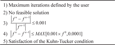
On the other hand, the gradient-free optimization method does not require sensitivity information, and depends only on the function evaluations to find the global minimum of the objective function. A pattern search algorithm or nonlinear SIMPLEX [14] uses heuristics, based on the geometric configuration of a simplex; while a genetic algorithm or evolutionary algorithm [15] is a nature-inspired, probabilistic method. However, due to its expensive computational cost, related to a relatively large number of function evaluations, the gradient-free method cannot handle many design variables, with their number typically limited up to twenty, or so. But for the functions of which one cannot compute the gradients at all design points, or where it is very difficult to compute the derivative values, the gradient-free methods are the practical choice of design methods, and the computational cost is reduced, if used in combination with the approximation model [16]. Various criteria can be used to terminate the design iterations, and locate the minimum of the function. Termination criteria of the optimization algorithms are listed in Table 1.
[Table 1.] Termination criteria during design optimization

Termination criteria during design optimization
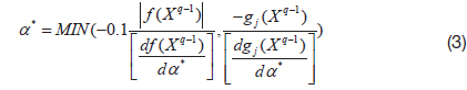
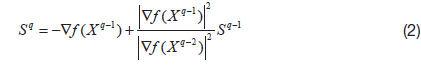
In the current design framework, various optimization algorithms are supported, as listed above. For example, the MFDA (Modified Feasible Direction Algorithm) [13], which is one of the famous gradient-based optimizers, describes the direction vector S at

And, the optimum step size is determined first, by approximating the
The MFDA is mainly used for the airfoil shape design framework. In the following sections, the descriptions of details for the design framework are focused on the MFDA-based design framework.
We introduce two famous methods, which demonstrate different characteristics, in terms of the accuracy and the computational efficiency, to compute the function derivatives: a conventional finite-difference method, and a complex-step derivative approximation
2.2.1 The Finite-Difference Method
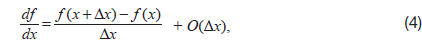
The finite-difference method is the simplest and most intuitive method. It is derived from the Taylor series expansion, by truncating higher order terms. A first-order forward-difference is written as below.

where,
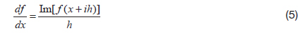
2.2.2 The Complex-step Derivative Method
This is a technique that estimates the sensitivity of a function, using the complex step. It is derived from the Taylor series expansion, by using the complex step,
3. Aerodynamic Analysis through Web-based CFD: EDISON_CFD
The method of CFD analysis is used to solve flow governing equations. Both inviscid Euler and viscous Navier-Stokes (NS) equations are solved. A discretized form of the NS equations is as follows.
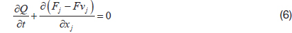
where,
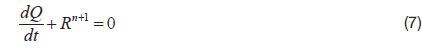
A basic cell-centered finite-volume method is used for spatial discretization of the equation. The solutions are advanced in time, through numerical time integration. Depending on how to linearize the convective term of Eq. (6), Roe’s FDS (Flux Difference Splitting) [18], modified Roe’s FDS [19], AUSM, and AUSMPW+ [20] are implemented. Mathematical details of each method are found in reference papers, and can be omitted here. A high order scheme, such as MUSCL (Monotone Upstream-centered Scheme for Conservation Law), is also available, by realizing a TVD (Total Variation Diminishing) approach, and prevents the spurious oscillations of the solution around the discontinuous and shock regions. A flux limiter is also implemented, to complement the low-order accurate flux discretization scheme. A residual of the space discretization is reduced, until the solution converges through the time-integration, as the form of

The explicit Euler method, multi-stage Runge-Kutta method, and implicit LU-SGS [21] are implemented. Also, viscous flux terms are solved by a central-differencing scheme. Various turbulence models are available, including standard
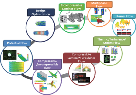
Both incompressible and compressible flow solutions are possible for a wide range of Mach numbers (from subsonic, supersonic to hypersonic). Complicated flow features, including multi-phase flow, thermal flow, and Stokes flow, are also resolved in the current framework of EDISON_CFD. Both internal and external flows are computed, to solve diverse types of fluid mechanics problems, including pipe and cylinder flows. Flow analysis of both laminar and turbulent conditions is carried out for a wide range of Reynolds number, and several transition models to predict the flow separation on the surface are implemented, as well. Fig. 1 shows the graphical schematic of the EDISON_CFD applications to various problems.
3.2.2 Parametric Surface Definition
Although one-time flow analysis requires a set of a fixed CAD model and a corresponding mesh for the configuration of interest, a design optimization requires different surface geometry at each design step, since the design produces a new set of design variables that have to be translated into shape modification. Therefore, smooth variation of the boundary surface and mesh deformation conforming to the surface variation is critical in the overall design process. Subsequently, flow analysis at each design step is required in a fast and automatic manner, for the new design candidate.
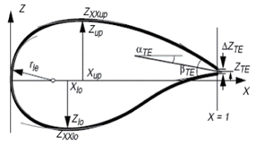
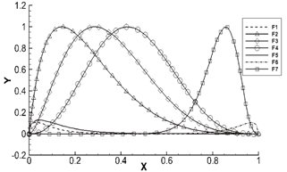
Surface variations are performed with respect to a different set of design variables, in two ways: 1) by explicitly changing the value of the parameters that initially define the surface boundary, or 2) by imposing arbitrary variations on the direction normal to the surface, which create implicit variations in shape. The surface variation through the control of the shape-related parameters requires an additional process, called profile fitting, to retrofit the approximate solution to the initial shape. A polynomial equation for a simple NACA airfoil, PARSEC [26], and NURBS [27] can directly have a parameterized relationship, to define the airfoil surface. The design parameters of PARSEC are shown in Fig. 2. On the other hand, a direct variation of the surface, by superposing the variation function onto the original surface, allows more flexible representation of the surface variation. The Hicks-Henne bump function [28] is a representative method in this category. A brief mathematical formulation is:
A careful consideration is required to choose the surface shape definition function, because it characterizes the design space, in terms of variation bounds and its dimension. In the current design framework, various types of shape definition functions are included, such as the polynomials for NACA 4-digit airfoil, PARSEC, NURBS, and Hicks-Henne bump functions. Users are able to correspondingly choose the appropriate shape definition method.
3.2.3 Mesh Generation and Dynamic Deformation
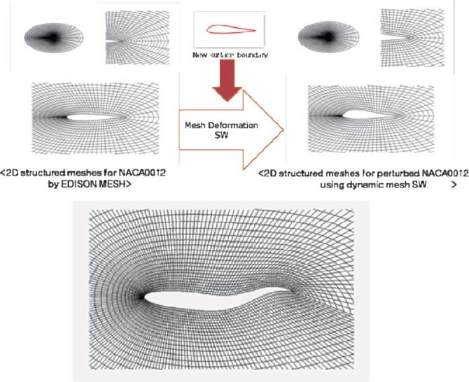
A pre-processing module of e-Mega is integrated into the EDISON_CFD solver, to generate computational grids for a user-defined arbitrary geometry. Both structured and unstructured mesh generators are possible; but we mostly use the structured mesh generation module in the current study, for its simplicity and efficiency at grid generation time. The clustering of mesh points in an arbitrary direction is possible, and various types of smoothing, including elliptic and parabolic differential equation solvers, are available to enhance the grid quality around the clustering area of the near-body, and the region of high pressure gradient.
Another key aspect to an efficient design is smooth mesh deformation, conforming to the surface variation. Automatic and dynamic mesh deformation that preserves the initial mesh quality is very important, as it does not require new mesh generation for a different geometry, at each design iteration. In this study, trans-finite interpolation (TFI) [29] is applied, to handle shape modification. The TFI method is a technique of dynamic mesh deformation for structured grids, and propagates the variation of surface nodes, by interpolating the neighboring mesh points. Moreover, a technique for handling large deformations near trailing edges in an O-type mesh is additionally implemented, and shown in Fig. 4. From a trailing-edge node to a far-boundary node, a 3rd-order polynomial with a pre-specified boundary condition is used to enhance the mesh quality. Then, a redefined edge is propagated to the whole mesh system, by solving an elliptic equation. The mesh deformation technique in this study is validated by undulatory airfoil motion [30], as shown in Fig. 4. Despite considerably large deformations, compared to a typical deformation during the design process, the mesh deformation and quality-enhancing techniques used in this study can effectively handle it.
4. Design Optimization Framework: EDISON_ Design
4.1 EDISON and EDISON_Design Portal Systems
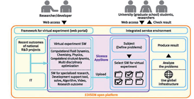
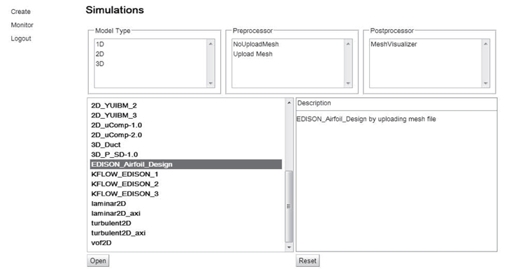
The EDISON portal system is a web-based simulation environment for engineering education and research, and is currently used in many domestic universities as an e-learning tool, for the courses of fluid mechanics and aerodynamics [8]. As can be seen in Fig. 5, one of the important features is that computing resources for the simulations are remotely provided with the users, and controlled by the national supercomputing center. The students can access the high-performance computers through the EDISON portal system, using their PC, which serves as a terminal to the supercomputing center. Users log on to the website through an Internet connection, and choose the CFD flow solvers and input parameters for the flow condition, and the job is launched remotely, via the portal system. Once the job is completed, the student can visualize the flow field directly in the portal system, or download the solution files to local storage. The user does not need to consider the expenses of purchasing and operating computing devices.
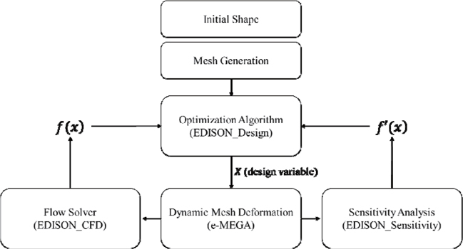
A design optimization framework of EDISON_Design is implemented in the EDISON portal [8], as one of the submodules. Its major advantage is to integrate the CFD flow solver of EDISON_CFD as a main modeling and simulation (M&S) tool of the design, for a high-fidelity flow solution. Fig. 6 represents an overall schematic of the EDISON_Design framework, and the interfaces among the individual modules are shown inside the framework. It includes a geometry kernel for surface definition and variation, dynamic mesh generation and deformation, flow analysis through the CFD solvers, and mathematical optimization algorithms for computing the search direction and step length. As the design proceeds through the design steps, a set of the design variables are updated, and represented as a new geometry; and corresponding mesh deformation and subsequent flow solutions are carried out in the EDISON_Design framework. Most of the computational cost is for the CFD flow solutions in function evaluation, and its derivative computation to determine the search directions. The whole design process is fully automated, through linked information for their input and output data, which makes the current framework particularly more advantageous for large scale problems involving many design iterations. The automatic design procedure and its detailed information are behind the GUI, which is particularly attractive for those users without much a prlori knowledge of mathematical design theory.
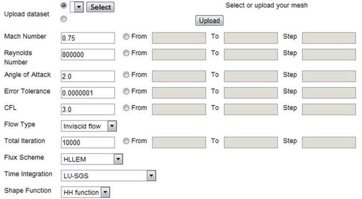
The available surface definition and variation algorithms for a two-dimensional airfoil are: PARSEC, Hicks-Henne bump functions, and NURBS representation. Also, the available optimization methods and sensitivity methods are summarized in Table 2, along with the available CFD solver types. A selection of the various choices of the EDISON_CFD solvers and EDISON_Design parameters is done through the GUI (Graphic User Interface) of the EDISON portal system. Fig. 7 and Fig. 8 show the GUI format of the EDISON environment for flow simulation and the corresponding input parameter set-up, respectively. Mach number, angle of attack, and the Reynolds number are options associated with the incoming flow conditions. Additionally, spatial and temporal discretization schemes of the CFD solvers, and the CFL (Courant-Friedrichs-Lewy) number can be chosen with flexibility, depending on the level of user’s knowledge of flow solvers. If the user is new to the numerical analysis of flow governing equations, default values are provided. For graduate students, they can have more options in generating meshes, and solving the PDE of the flow governing equations.
[Table 2.] Optimization methods and sensitivity analysis method
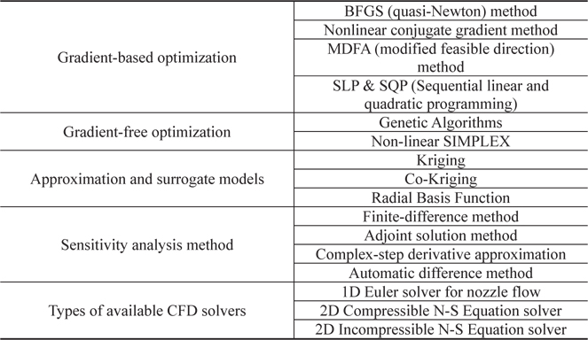
Optimization methods and sensitivity analysis method
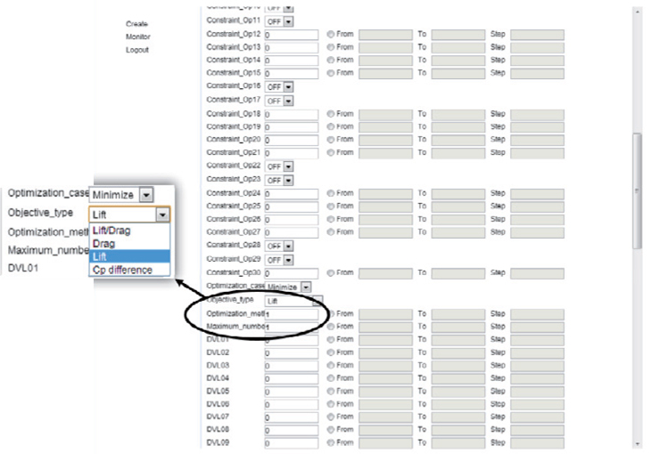
In the optimization through EDISON_Design, numerous choices of the shape definition types, optimization algorithms, the objective function, and the constraints definition are available, as shown in Fig. 9. Like EDISON_CFD, the level of the user’s expertise in CFD analysis and design optimization is taken into consideration. For advanced users, detailed input parameters for the optimization algorithm can be selected, without the default options. The flexibility of the proposed design framework of EDISON_Design is mainly attributed to the capability of the EDISON_CFD solvers that can handle various types of flow problems, in the fields of aerospace, mechanical, civil, ocean engineering. Though the applications are different with the individual geometry of the configuration of interest and a proper EDISON_CFD solver for specific flow conditions, a basic approach for the design optimization is common for all problems. However, depending on the complexity of the problems, and the size of the computation domain, the choice of the design strategy including the optimization algorithms, and definition of the design variables, has to be different, in the usage of the EDISON_Design. The resultant accuracy and efficiency of the design solutions have to be addressed at the same time.
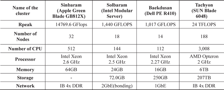
Another advantage of the current design framework is the provision of powerful computing resources for multiple users. For complicated problems with a large computation domain, parallel computation is needed, and made available through the high-performance computing environment. The national supercomputing center of KISTI (Korea Institute of Science and Technology Information) provides computation resources with various user interface options of GUI, via the web-based connection. Depending on the scale of the problem, and the size of the computational mesh, a different level of parallelization is recommended to the user. Load balancing is carried out, to handle a large number of users simultaneously. The following are the available computing resources, and their detailed performances, in terms of
[Table 3.] Computer clusters that are provided for the EDISON users

Computer clusters that are provided for the EDISON users
5. Educational Applications: Aerodynamic Shape Optimization for Airfoil
As the main purpose of the current study is to solve design problems of aerodynamic shape optimization, we take an example of a two-dimensional airfoil to reduce wave drag at transonic flow conditions. Although the EDISON_DESIGN framework itself can be applied to the design problems involving both two- and three-dimensional complex geometries, we demonstrate a two-dimensional design problem that can be taught in undergraduate design courses. This problem was discussed in the courses of Aerospace Systems Design, and Advanced Numerical Analysis. Students often want to design transonic aircraft, which fly at a transonic Mach number that is in the neighborhood of the drag-divergence Mach number. The design of a supercritical airfoil that reduces the strength of the shock on the airfoil is critical. Thus, the design of an airfoil shape that has low wave drag becomes a good design practice for the students to understand the fundamentals of transonic flows, and to learn mathematical design optimization procedure. The design problem has a practical meaning for aircraft design courses.
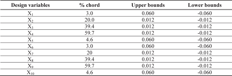
Drag minimization of an airfoil in the transonic flow regime was conducted. Geometrical constraints of the maximum thickness ratio and area of the airfoil, as well as performance constraints on lift coefficient are imposed, and a design vector is bounded with lower and upper limits, and creates a feasible region of the design space. For the geometric design variables, 10 weighted values of the Hicks-Henne bump function are set, 5 each for the upper and lower surfaces of the airfoil respectively, to impose surface perturbations. Their locations and bounds are shown in Table 4. A mathematical formulation of the problem definition is stated in Table 5. The lift coefficient is allowed to increase, to result in a better lift-to-drag ratio of the airfoil. The maximum thickness ratio is set to vary with both positive and negative variations of 6–22% that of the baseline. In addition, the lower bound for the lift coefficient is set to be that of the baseline, so that it increases the efficiency of finding the optimum solution.
[Table 4.] Bounds of Design Variables

Bounds of Design Variables
[Table 5.] Problem statement of direct design optimization
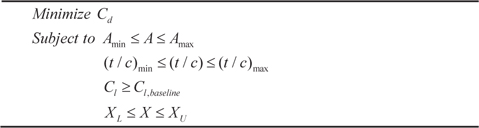
Problem statement of direct design optimization
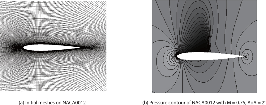
Two-dimensional, compressible Euler equations, which govern inviscid fluid flows, are solved, to analyze flow around the airfoil. For the spatial discretization of the governing equations, a RoeM scheme is used, and an implicit LU-SGS method is chosen for the temporal discretization. Moreover, fluid analysis using the Navier-Stokes (N-S) equation is also conducted, to verify differences between flow solutions calculated by the Euler and N-S solvers. For the turbulent model, Menter’s
5.2 Drag Minimization of Airfoil at Transonic Flow
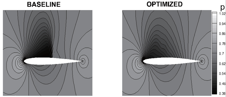
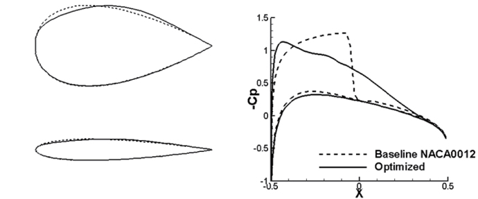
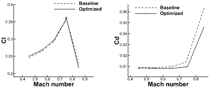
Given the design problem in Table 5, optimization is carried out using the MFDA algorithm, with the gradient values calculated by the finite-difference method. After 128 design iterations, the results of drag minimization of NACA0012 airfoil are obtained that satisfy the pre-specified convergence. The optimized airfoil shape is shown in Fig. 11, and compared with the baseline. Comparisons of the pressure contours of both airfoils are also shown in Fig. 12. Aerodynamic force coefficients are also summarized in Table 9. The leading edge becomes slightly thinner, and a minor camber is added toward the rear region, after the mid-chord of the airfoil. Strong shock on the upper surface of the airfoil is reduced, and decreases the drag coefficient from 105 counts to 7 counts. This reduction is dramatic, considering the minor changes in the airfoil shape; however, previous sensitivity analysis shows this region to be very sensitive to shock strength and wave drag.
To verify the aerodynamic improvement at off-design Mach numbers, flow simulation is carried out at the wide range of Mach number from 0.5 to 0.85, and the corresponding drag is plotted in Fig. 13. This shows that the designed airfoil also improves aerodynamic performance in the off-design condition, beyond the drag-divergence Mach number [29]. In other words, drag reduction is possible for a wide range of Mach numbers, beyond the design Mach number of 0.75, up to Mach = 0.85. It is also noticeable that the lift coefficient is almost constant, for a wide range of Mach number. In conclusion, following the whole process of the numerical design of an airfoil can help students to understand the physics of the flow around an airfoil, as well as the standard procedures of design in the general engineering field.
A computational design framework for airfoil design is developed for education and research purposes, in the engineering field of fluid mechanics. It is notable that the framework software uses the CFD solver as a functional evaluation tool. Owing to the high-fidelity analysis of CFD flow solution methods, the design framework can be more sophisticated. In general, the high-fidelity analysis of CFD requires a high computational cost. However, web-based CFD analysis helps the design framework to be more efficient. Students and researchers can investigate specific flow physics more accurately, and find a more credible optimum solution, than with low-fidelity analysis. The sub-elements of the framework, such as the geometry kernel, mesh deformation, optimization algorithm, and flow analysis, are robustly and organically integrated. In future work, we will further expand the design framework to many other engineering applications, for both educational and research purposes. In addition, the latest design methodologies will be implemented, such as meta-model-based design, and the adjoint variable method. Advances in software development will help us to add more diverse education contents to provide a theoretical background to the users, and a more user-friendly environment will be developed, using a graphic user interface (GUI).


![Various applications of EDISON_CFD [8]](http://oak.go.kr/repository/journal/13486/HGJHC0_2013_v14n4_297_f001.jpg)

![Overview of integrated research: parametric study services [8]](http://oak.go.kr/repository/journal/13486/HGJHC0_2013_v14n4_297_f005.jpg)