In sensor networks, a large number of inexpensive, lowpower communication sensor devices with one or more sensing capabilities are deployed in a sensor field, providing physical sensing phenomena, processing them, and communicating this information to other sensors. These sensors are battery-powered and the network lifetime is a crucial concern for sensor networks. Collecting measurements from many sensors and transmitting them for various tasks (e.g., localization, tracking targets, and temperature monitoring) will reduce the lifetime of a network. Thus, the sensing tasks should be able to minimize the number of sensors involved in order to prolong the network lifetime. This will motivate the selective use of the most informative sensors, resulting in a reduction of the number of sensors in operation.
In the scenario of localization using wireless sensor networks, the localization accuracy can be significantly improved by selecting the most informative sensors [1-3]. For example, the entropy-based heuristic approach proposed in [1] greedily selects the next sensor in order to reduce the overall uncertainty. The authors of [2] focus on finding the best set of sensors that maximizes the localization accuracy, under the assumption of a known uncertainty region for the source location; further, they present analytical bounds on the performance of their sensor selection algorithm. In [3], the author addresses the sensor selection problem when the quantization of measurements is taken into account and shows that this sensor selection problem can be treated as a rate allocation problem where the goal is to allocate the rate to each sensor so as to minimize the localization error. To solve this problem, the generalized Breiman, Friedman, Olshen, and Stone (BFOS) algorithm (see [4]) is applied with the rate-distortion (R-D) calculation for each candidate rate allocation.
However, most of the existing algorithms suffer from a high computational complexity, since the sensor networks consist of a large number of sensors and the process of selecting sensors must be executed online whenever every event of interest occurs. Thus, fast and powerful sensor selection algorithms are required to facilitate the practical applications of large sensor networks. In this paper, we propose a simple geometry-based sensor selection algorithm by utilizing only the information of sensor locations. Motivated by the observation that sensors clustered together tend to generate redundant information [3], we seek to find a set of sensors that are located at the maximum distance from each other. More specifically, we search the best set of sensors that maximizes the average distance between the sensors within the set. Furthermore, in order to accelerate the selection process, we propose an iterative sequential search algorithm without losing optimality, instead of directly conducting an exhaustive search of sensors over the sensor field. We show that the proposed algorithm reduces the average distance in each iteration, ensuring the convergence of the algorithm. Our experiments demonstrate that the proposed sensor selection achieves a significant performance improvement as compared to random sensor selections and exhibits a performance close to that of the exhaustive search among sensors over the sensor field.
Throughout this paper, it is assumed that each sensor can obtain a noise-corrupted measurement, such as signal energy or temperature using actual measurements (e.g., time-series measurements or spatial measurements) and there are only one-way noiseless communication channels from the sensors to the fusion node; i.e., there is no feedback channel, and the sensors do not communicate with each other (no relay between sensors).
The rest of this paper is organized as follows: The problem formulation is given in Section II. The geometrybased sensor selection algorithm is explained in Section III. The iterative sequential algorithm is summarized in Section IV and the proposed algorithm is applied to the acoustic amplitude sensor system for source localization, which is introduced in Section V. Simulation results are presented in Section VI and the conclusion is stated in Section VII.
Within the sensor field
where
We believe that this formulation is general and captures many scenarios of practical interest. Each scenario will obviously lead to a different sensor model
III. GEOMETRY-BASED SENSOR SELECTION ALGORITHM
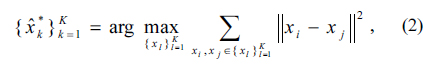
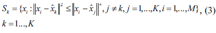
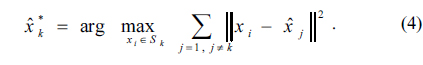
It is observed that sensors clustered together tend to send redundant information to a fusion node [3] and thus, a good strategy would be to select sensors that are at the maximum distance from each other. To be specific, we seek to search the best set of
where the distance ║
In search for the best set, we take an iterative sequential approach rather than an exhaustive search to make the algorithm practically applicable to large sensor networks (
where
Note that this search should be conducted under the constraint of the distance range. It is obvious that the construction of
The proposed algorithm is iteratively executed over all sensors
Algorithm 1: Geometry-based iterative design algorithm.
Step 1 : Initially, set iteration index n = 1 and choose randomly K out of M sensors to construct a set, Step 2 : Construct K regions, Sk , k = 1, …, K by using Eq. (3).Step 3 : Find the k-th sensor from its corresponding region Sk that maximizes the average distance by using Eq. (4).Step 4 : Set = and repeat Step 3 for the other K − 1 sensors.Step 5 : Set n = n + 1 and construct the new set Step 6 : If Vn-1= Vn , then stop; otherwise, go to Step 2.
Note that the proposed iterative algorithm suffers from the presence of numerous poor local optima depending on the initialization of set
V. APPLICATION TO ACOUSTIC AMPLITUDE SENSOR CASE
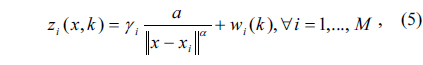
As an example of an application of the proposed algorithm, we consider the acoustic amplitude sensor system for source localization where an energy decay model of sensor signal readings proposed in [6] is used for localization. This model is based on the fact that the acoustic energy emitted omni-directionally from a sound source will attenuate at a rate that is inversely proportional to the square of the distance in free space [7] and was verified by the field experiment in [6] and used in [8-10]. When an acoustic sensor is employed at each sensor, the signal energy measured at sensor
where the parameter vector P
The
>
A. Location Estimation Technique Based on Quantized Data
Clearly, for z
While specific g(.) choices depend on the sensor model
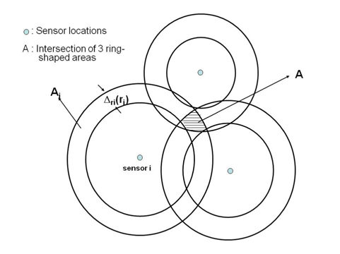
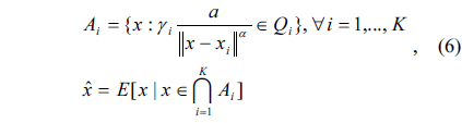
More specifically, here, we consider the estimator g(.) that performs energy-based source localization by using quantized data. Note that the localization algorithm to be explained in this section is designed for the high signal-tonoise ratio (SNR) regime (σi = 0) but will also provide a foundation for the localization based on noisy quantized data [9]. Since each quantized sensor reading corresponds to a region where a source is located, all quantized sensor readings lead to a partition of a sensor field obtained by intersecting the regions corresponding to each sensor reading. The localization based on the quantized sensor readings is illustrated in Fig. 1, where the ring-shaped area,
where
In the experiments, we consider an acoustic sensor network where
The sensor selection of the proposed algorithm is compared with many sensor selections
>
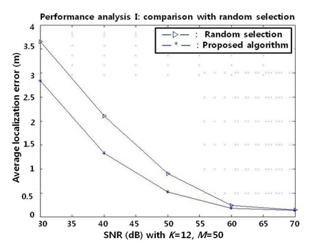
A. Performance Analysis I: Comparison with Random Sensor Selections
In this experiment, 100 different sensor configurations are generated for
>
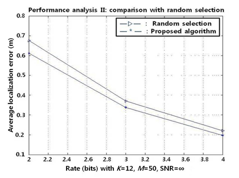
B. Performance Analysis II: Effect of Quantization
One hundred different sensor configurations are generated for

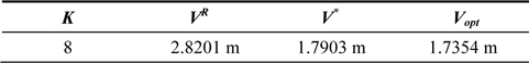
Comparison of the selection techniques, VR, V* with optimal solutions, and Vopt for K = 8, M = 20, and SNR = 40 dB
>
C. Performance Evaluation: Comparison with Optimal Selection
The proposed algorithm is evaluated by comparing its selection with the optimal selection
Thus, for each configuration, the localization errors are computed for
In this paper, we have proposed a geometry-based sensor selection algorithm optimized for large sensor networks. To achieve low complexity, we suggest the use of the average distance between sensors within a set as a metric to be maximized and propose an iterative sequential search algorithm to find the best set of sensors that maximizes the average distance. This algorithm was applied to an acoustic sensor network for source localization and was shown to perform quite well in comparison to random sensor selections. In the future, we will continue to improve the proposed algorithm in terms of performance and complexity.