Interest on offshore energy resources has been increasing globally, especially in Brazil, India, China, and other developing countries. The marine world in 2030 will be almost unrecognizable owing to the rise of emerging countries as mentioned, new consumer classes and resource demand (Fang et al., 2013). As development activities for energy demand move to deepwater, many offshore pipelines to transport oil and gas will be installed. The clay soil on seabed below installed pipelines ranges from very soft to very stiff soil. This paper deals with soft and very soft clay soil and the pipelines will be embeded further into the soft soil. The exact behavior between a pipeline and soil is not known. The heaved soil and resistance forces are hence important aspects. It is important to properly model pipe-soil interaction effects (Bai and Bai, 2005). Pipe embedment depth by pipesoil interaction has become critical design parameter to design offshore pipeline such as free span and thermal expansion as well as on-bottom stability. On-bottom stability analysis that a pipeline maintains stability on seabed against hydrodynamic load of wave and current has to be considered with a relevant pipe-soil interaction analysis.
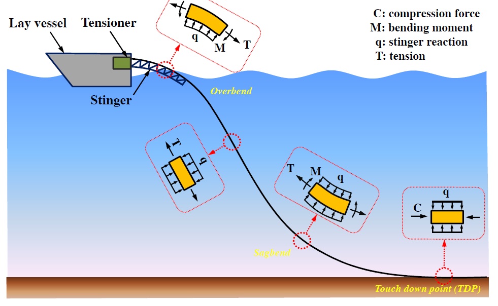
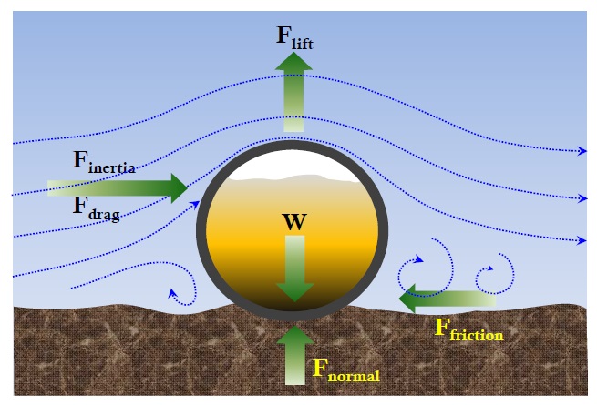
The pipelines are under the combined loads such as bending, axial force, and external pressure during installation due to the dynamic vessel motion. At TDP, the seabed disturbance will occur by the dynamic pipe-soil interaction. A typical s-lay configuration and applied pipeline loading during installation is presented in Fig. 1.
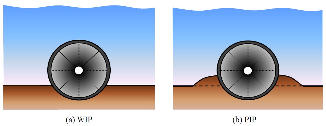
Studies on pipe-soil interaction and assessing penetration depth have been progressing lately. Verley and Lund (1995) developed pipe-soil interaction models on clay soils considering penetration effects of pipe subjected to oscillatory forces in waves based on model test data and this formula was adapted in DNV-RP-F109. White and Cheuk (2008) studied soil resistance on seabed pipelines during large cycles of the lateral movement for realistic soil behaviors. Randolph and White (2008b) and Merifield et al. (2009) present pushed-in-place (PIP), taking into account of combining the vertical and horizontal loading using a heaved soil model. Before these studies, the model based on wished-in-place (WIP) considering relations only between the vertical load and normalized pipe penetration was used. The WIP and PIP models are illustrated in Fig. 2.
The environmental loads on the embedded pipelines are reduced on soft clay. If an exact initial penetration depth can be calculated, an optimized required submerged weight can be derived easily. Currently, no methodology has developed considering simultaneously both of the dynamic pipeline installation and the pipe embedment at TDP. Thus a new proposed procedure was developed in this study. The details of the procedure are described in the next chapter.
In this study, the recent trend for the on-bottom stability analysis was investigated and a case study was performed using the proposed new procedure. Analysis results between seabed penetration depths with dynamic effect and without dynamic effect were compared.
A NEW PROCEDURE OF ON-BOTTOM STABILITY ANALYSIS
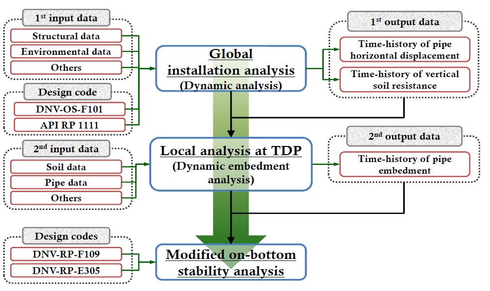
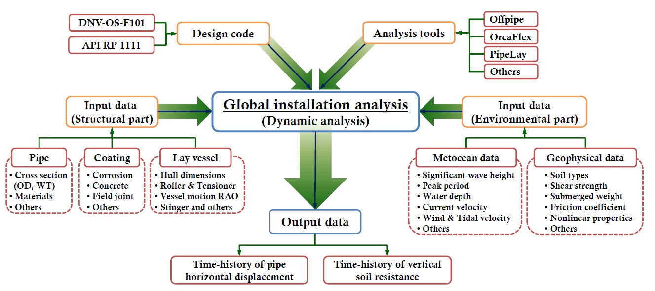
Fig. 3 shows the proposed new procedure for the on-bottom stability with dynamic effect of offshore pipeline installation. The analysis procedures are made up three steps such as global pipelay analysis, simulation of dynamic local pipeline embedment at the TDP, and modified on-bottom stability design. Details on each step are described in the subchapters. The time histories of horizontal displacement and vertical soil resistance at TDP are calculated through global pipelay analysis using pipe properties, environmental data, and others. The time histories of horizontal displacement and vertical soil resistance were used for input of local pipe-soil interaction analysis with a finite element method (FEM). The maximum value among pipe embedment depths by local dynamic analysis was used for an initial penetration depth, the modified on-bottom stability analysis based on DNV-RP-F109. The calculation result based on design codes considering the dynamic penetration depth from FEA can be used for an optimum on-bottom stability design.
>
Global installation analysis
The commercial pipeline installation programs are based on FEA and calculated the stress, strain, touchdown length, departure angle, and soil reaction force at TDP. Installation method of the s-lay was used for the present study. General procedure and details of the global analysis are summarized in Fig. 4. The DNV-OS-F101 (DNV, 2012) for design criteria was used to check the allowable stress and strain. The OFFPIPE software as an analysis tool was used in this study. The background of OFFPIPE software could be referred to OFFPIPE manual (OFFPIPE, 2013).
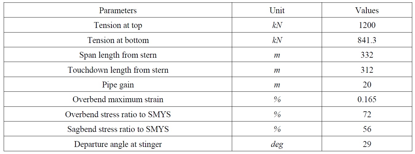
The environmental input data include waves, currents, water depth, and soil shear strength, submerged weight of soil, and friction coefficient. The lay vessel information incorporates hull dimension, locations of rollers and tensioners, configuration of stinger, and vessel response amplitude operator (RAO). The installation analysis was divided into two steps: static and dynamic analyses. Important parameters in this analysis are summarized in Table 1. Results by static analysis were checked with design criteria and then dynamic analysis was performed. Time histories of horizontal displacement and vertical soil resistance were obtained by the dynamic pipelay analysis.
[Table 1] Global installation analysis parameters from OFFPIPE.
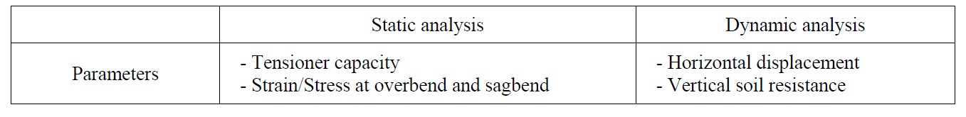
Global installation analysis parameters from OFFPIPE.
The purpose of the local analysis is to estimate initial pipe embedment depth considering the dynamic loads from global pipelay analysis. The procedure of local analysis is illustrated in Fig. 5.
The most important information to obtain pipe embedment depth by local analysis is soil data of seabed. Data such as shear strength, Young’s modulus, and Poisson’s ratio for soft clay should be entered exactly though in-situ testing. Plastic properties such as sensitivity and soil ductility are also important. There are FEA tools such as Abaqus and ANSYS for the pipe-soil interactions. Elastic perfectly plastic soil models including Mohr-Coulomb, Tresca, and von-Mises criteria and elasto-plastic soil model including modified Cam clay are used for many geo-engineering problems.
Recently, researches on pipe-soil interaction behavior have been conducted actively and many constitute equations which are expressed mathematically about stress-strain relation, initial yield strength, hardening, and softening on soil behavior are being developed. For example, Tresca criteria with the strain-softening was used for the pipe-soil interaction analysis and research work including tests was actively performed by Einav and Randolph (2005), Zhou and Randolph (2007), Wang et al. (2009), Chatterjee et al. (2010) and many others.
The empirical expression of shear strength for tresca constitutive model with exponential strain softening relationship is as follow (Zhou and Randolph, 2007; Wang et al., 2009).

where,
Su0 = Intact undraind shear strength, ( = Sum + k ⋅ z );
k = Strength gradient;
z = Soil depth;
δrem = Fully remoulded strength ratio, ( 1/= St);
St = Sensitivity;
ξ= Accumulated absolute plastic shear strain;
ξ95 = Cumulative absolute shear strain required to cause 95% reduction.
>
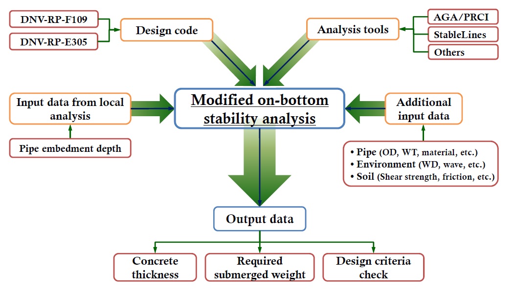
Modified on-bottom stability analysis
The design procedure of modified on-bottom stability is presented in Fig. 6. General environmental data for each condition are selected as follows (Guo et al., 2004).
Installation condition: empty pipes with 1-year period environment
Operation condition: product filled pipes with 10-years or 100-years period environment
A design of on-bottom stability was performed according to following. Firstly, environmental criteria for the 1-year, 10-
In this study, on-bottom stability analyses were performed based on the modified analysis and DNV-RP-F109. The details on this design code are explained in chapter 3 of DNV-RP-F109.
A CASE STUDY ANALYSIS OF ON-BOTTOM STABILITY
The on-bottom stability analyses were performed based on above mentioned new procedure including global and local analyses of offshore pipelines and modified application of DNV-RP-F109.
>
Global installation analysis
Input data
A 32-
[Table 2] 32-inch pipeline data.
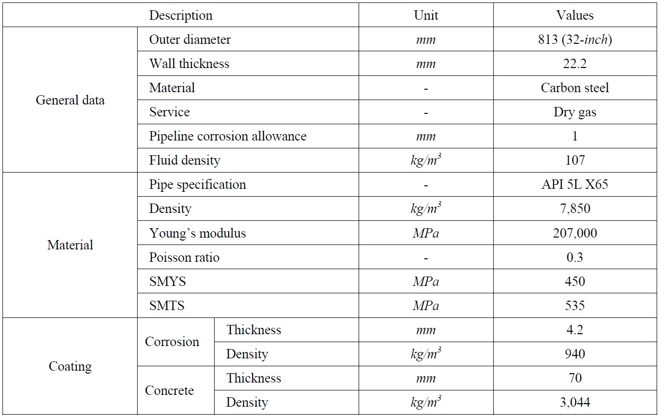
32-inch pipeline data.
Environmental data.
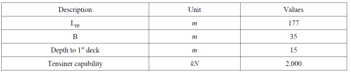
Lay vessel data.
As mentioned before, dynamic pipelay analyses were performed by using OFFPIPE and its input file requires following data: pipe, coating, barge, supports including roller and tensioner, stinger geometry, and tension data for static analysis. In addition, time limits for analysis, wave, and laybarge motion RAO data were required for the dynamic analysis.
Calculation method
The formulas for the static pipe stress during pipeline installation in OFFPIPE are as below. The tensile stress (
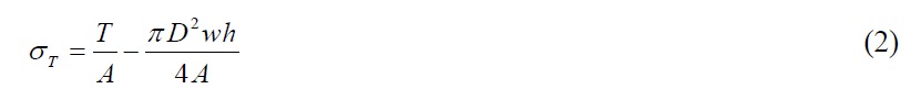
where,
The vertical and horizontal bending stresses (
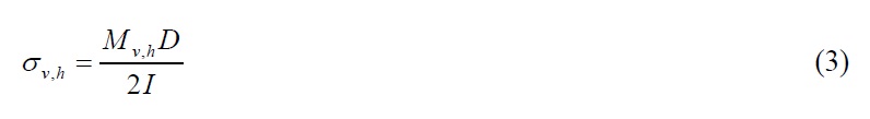
where,
The hoop stress (σh) in the pipeline is given by:
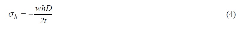
where,
The total or equivalent pipe stress (
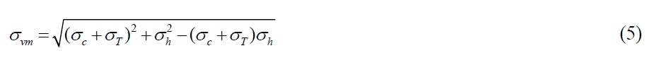
where,
For the soil effects, the seabed in OFFFPIPE is modeled as a continuous and elastic frictional seabed model. the vertical soil reaction as each point is given by:
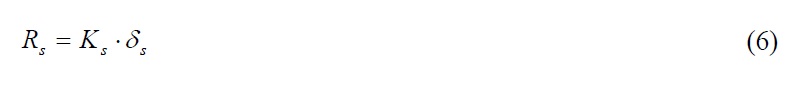
where,
The FEM is used for static and dynamic analysis in OFFPIPE and the solutions are also fully nonlinear. That is, it is to a numerical solution of the exact nonlinear differential equation of motion for beam subjected to large deflection and nonlinear material behavior. This FEM represents a nonlinear moment-curvature relationship for a large strain for a pipeline and effects of nonlinear boundary conditions for contacts. The numerical integration to solve equations of motion for the pipeline is used and the dynamic response to environmental forces and the wave by a vessel motion is calculated.
Design criteria in DNV-OS-F101
Check of allowable stress and strain was reviewed by DNV-OS-F101. Table 5 shows the simplified strain criteria of pipeline’s overbend in the design codes. In sagbend, the design code suggests that the equivalent stress criterion is below 87% of SMYS and this criterion covers both static and dynamic analyses.
[Table 5] Simplified strain criteria of pipeline??s overbend.
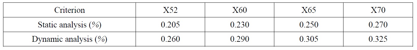
Simplified strain criteria of pipeline??s overbend.
Analysis results of the case study
Static analysis results of the case study are summarized in Table 6.
[Table 6] OFFPIPE static analysis summaries.
OFFPIPE static analysis summaries.
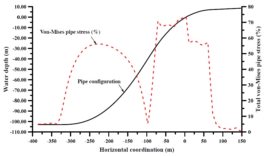
Result of required tension at top (safety factor, S.F. = 1.67) is below tensioner capacity. Results at overbend (S.F. = 1.52) and sagbend (S.F. = 1.55) are satisfied with the allowable laying criteria and are shown in Table 7. Fig. 8 shows the total pipe stress percent yield (%) throughout pipelay configuration during installation.
[Table 7] Results of static analysis of global pipelay.
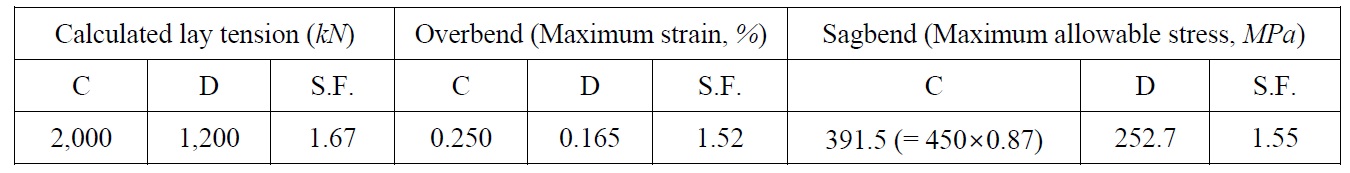
Results of static analysis of global pipelay.
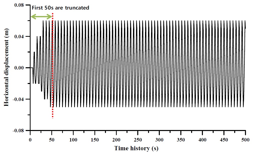
In check of overall static results, support reaction forces and vertical separations between rollers and pipe should be checked besides above stress/strain limit. After the force equilibrium state of the pipeline is converged by a static analysis, a dynamic laying analysis will be performed. Fig. 9 shows the time history of the lateral displacement at TDP for 500
Fig. 10 shows vertical soil resistances at TDP. The soil resistances vary with the pipe movements. The soil is under loads of 2.63
[Table 8] Results of dynamic analysis of global pipelay.
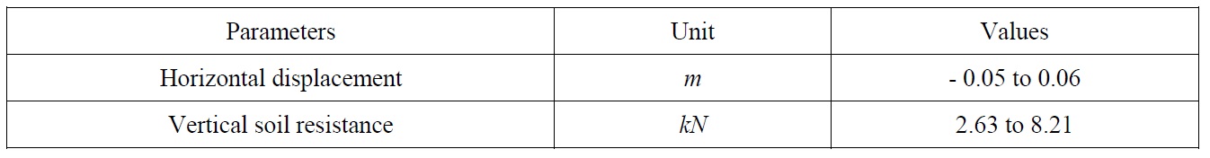
Results of dynamic analysis of global pipelay.
Input data
A pipe-soil interaction analysis was performed by a commercial finite element software Abaqus/CAE (Abaqus, 2011) and soil data in Table 9 and global installation analysis results were used for inputs.
[Table 9] Soft clay soil data.
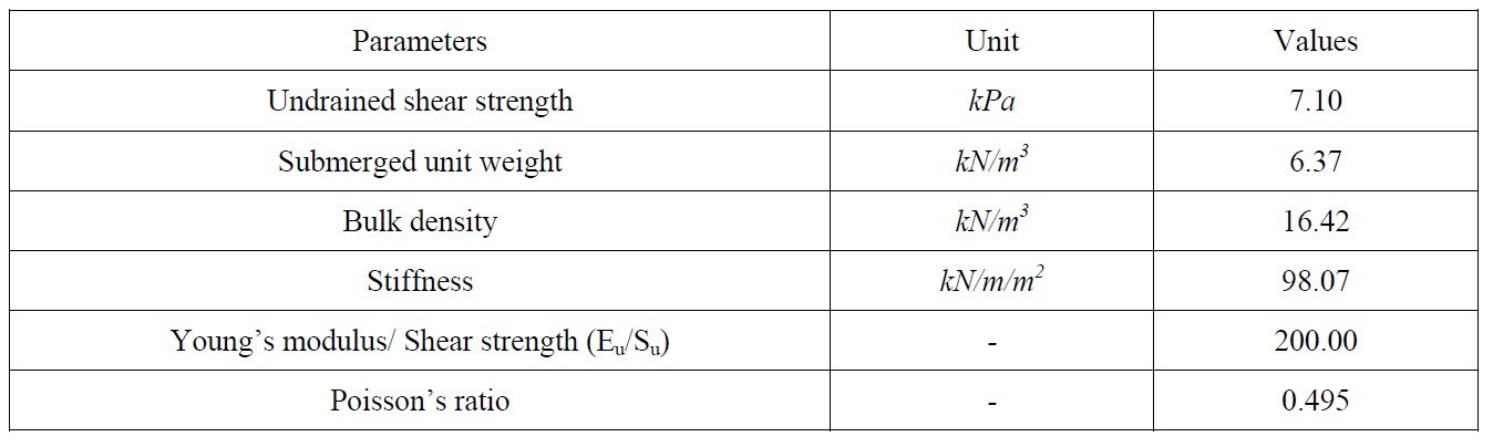
Soft clay soil data.
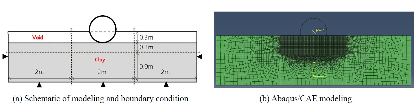
Finite Element Model
The coupled Eulerian-Lagrangian analysis technique was used for modeling large deformations in the analysis. The pipeline was modeled as a Lagrangian rigid body. Eulerian element was used for the soil because Lagrangian analysis for soil leads serious mesh distortion. In Eulerian domain, a void layer filled with zero strength and stiffness above soil domain was defined to allow the soil to flow into the initially empty Eulerian elements. Fig. 11 shows Abaqus/CAE modeling, boundary condition, and adaptive mesh. The portions of the pipe and soil interaction directly were generated with very fine meshes.
The loading condition was divided into two steps. A pipe settles down by applied vertical force at reference point at center of pipe mass in step 1. Then dynamic analysis was performed by applying lateral displacement time history resulted in global installation analysis in step 2. In the global dynamic installation analysis, the soil reaction force was range of 2.63 to 8.21
Soil constitutive Model
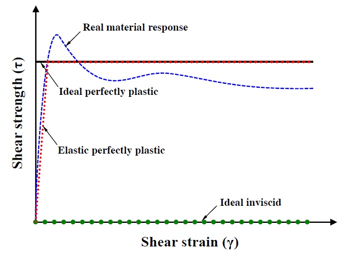
In this study, the elastic perfectly plastic soil model with Tresca failure criterion was used and the model is red dot line in Fig. 12. The concept of elastic perfectly plasticity is a simplified assumption of the complex plastic behavior of soils. This model is used in situation of loading of fully saturated clay soil using a total stress approach and requires the representative three material parameters; Young’s modulus, Poisson’s ratio, and undrained shear strength. The strength gradient term by soil depth was ignored in intact undrained shear strength.
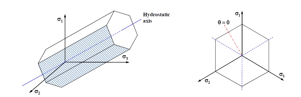
The Tresca failure criterion is used in geotechnical engineering to calculate the failure loads of clay soils deforming under undraind condition and same as the Mohr-Coulomb failure criterion with friction and dilation angles of zero. Fig. 13 shows the Tresca failure criterion in a three-dimensional stress space.
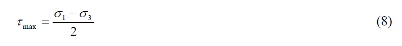
The intersection of the Tresca yield surface with a deviatoric plane creates a hexagon. The point of hexagon in triaxial compression and extension points results in singularities of the normal gradient to the yield surface. The Tresca failure surface can be expressed as:
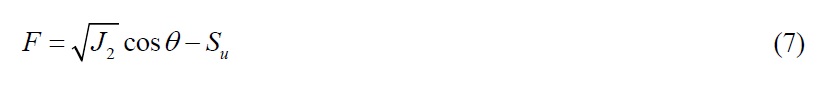
where,
When the relation of principal stress at each axis is
Analysis results
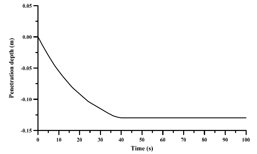
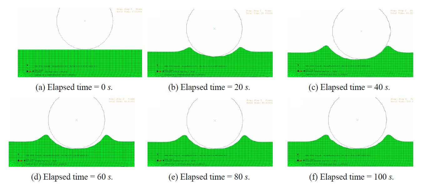
Figs. 14 and 15 show results on pipe-soil interaction behavior and pipe embedment depth by local analysis during 100
The 32-
Through pipe-soil interaction analysis, penetration depth of 129
>
Modified on-bottom stability analysis
Input data
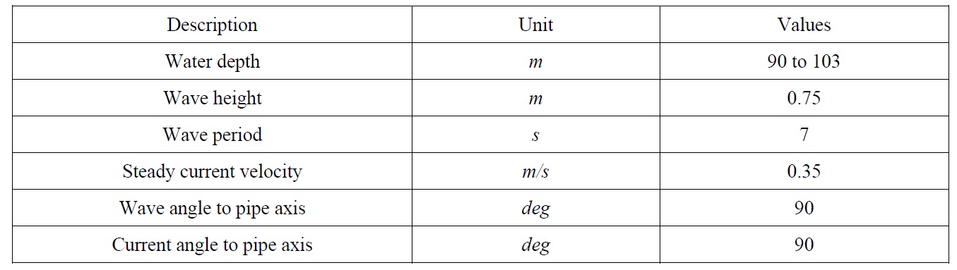
The water depths in this case study are from 90 to 103
[Table 10] Environmental data.
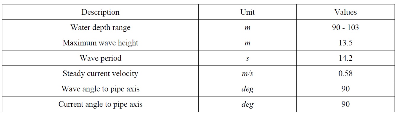
Environmental data.
Design code criteria
There are two methods in on-bottom stability design suggested by DNV-RP-F109 for the lateral stability. The former is generalized lateral stability method that displacement of pipeline is allowable to 0.5 (Lstable) and 10 times (L10) outside diameter. The latter, called absolute lateral stability method, do not allows displacement of pipe and considers environmental loads associated with a single design oscillation (maximum values).
Generalized stability method does not consider soil effects at seabed. In absolute lateral stability method, many soil effects including load reduction by permeable seabed, penetration, and trenching, passive resistance force, and friction coefficient are considered. Initial penetration depth calculated in local analysis has effects on calculation of load reduction and passive soil resistance force.
DNV-RP-F109, “on-bottom stability design of submarine pipelines”, uses formula for calculation of initial penetration depth from various experiment results by Verley and Lund (1995). This formula considers the penetration resistance without dynamic effects and is indicated in Eq. (9) (Randolph and White 2008a). However, this equation underestimates the penetration depth especially in soft clay and results in very unrealistic submerged pipe weight.
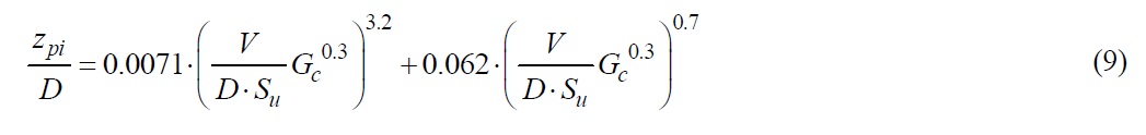
where,
z pi = Initial penetration depth; D = Pipeline diameter; V = Vertical force per unit length; Su = Shear strength;
Gc = Soil (clay) strength parameter (= Su / (D⋅γ s ) ); γs = Dry unit soil weight.
After initial penetration depth (
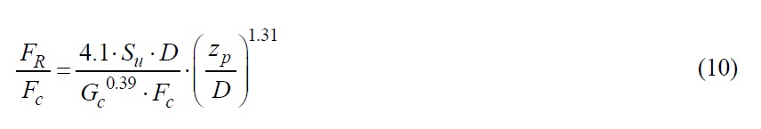
where,
FR = Passive resistance force; Fc = Vertical contact force between pipe and soil (= ws − Fz );
Required submerged weight (
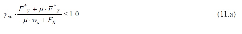
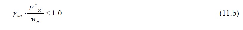
where,
γsc = Safety factor; F*Y = Peak horizontal load; F*Z = Peak vertical load; μ = Coefficient of friction by soil type;
ws = Pipe submerged weight.
Analysis results
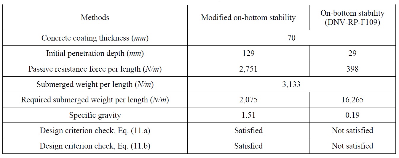
An on-bottom stability analysis was performed by above procedure and the results are summarized in Table 11. The results between initial penetration depths calculated by the present deign code and considering dynamic effects are compared.
Through above results, initial penetration depth which was calculated with effects of pipe-soil interaction on soft clay (FEA) is 129
[Table 11] Results of on-bottom stability analysis (Absolute stability method).

Results of on-bottom stability analysis (Absolute stability method).
In this paper, recent trends, analysis procedure, and importance on considering dynamic effect for on-bottom stability were investigated and studied and it was to help understanding on these through an applied example. Conclusions on performed results are summarized as follows.
•On-bottom stability of offshore pipeline on soft clay is very sensitive to the soil and pipe installation parameters.
• A new procedure of an on-bottom stability analysis especially on soft clay is proposed: from the global pipeline analysis for the dynamic time histories at TDP to the local FEM for the pipe embedment.
• The time history of lateral displacement of pipelines and vertical soil resistances at TDP can be obtained through global dynamic installation analysis.
• Using the results of global dynamic installation analysis, the behavior of pipe-soil interaction can be assessed by the local analysis using FEM. Pipe penetration depth was calculated with an elastic perfectly plastic clay model with Tresca failure criterion.
• Pipe embedment calculation by a local analysis was verified by an ROV inspection after the pipeline installation.
• Modified on-bottom stability analysis based on DNV-RP-F109 was carried out. Analysis results considering dynamic effect were resulted in about 4.5 times pipe embedment depth and about 7 times passive resistance force of analysis result based on static formula suggested in design code.
• Many studies on pipe-soil interaction, especially soft clay, and on-bottom stability have been carrying out. In case of soft clay, the effects of dynamic pipeline installation and embedment can be considered by the proposed method. This fact was included in the proposed design procedure presented in Fig. 3 through Fig. 6. This modified method was also approved by DNV (2011).