Intrusion detection is an important technology in computer defense; it can detect anomalous activity through feature matching. Portnoy [1] was the first to propose intrusion detection techniques based on cluster analysis using Euclidean distance; after identification, classification can be used to detect anomalies. However, there are some problems with these methods, such as weak self-adaptability, sensitivity to the initial value, vulnerability to the impact of noise and isolated points, and the easy of converge to local extrema among other defects. This may yield an unsatisfactory detection result with a low detection rate. Genetic algorithms (GAs) are used to simulate the natural mechanisms of a biological evolutionary randomized search algorithm. They are more suitable that processing with traditional search methods to solve complex optimization problems. GAs have strong global search capabilities, but they are weak for local search. Improving upon the traditional fuzzy C-means (FCM) algorithm, we use a GA to optimize the processing results. First, the data is divided into many subsets of data. Second, we use the FCM clustering algorithm to obtain the clustering center of each subset of data. Then we use a GA to optimize these cluster centers. As a result we can get an approximation of the global optimal cluster centers. Finally, we use this result as the initial value of the FCM algorithm. In this way, we combine the two algorithms for processing. Not only can we overcome the FCM algorithm’s sensitivity to the initial value and the problem of converging to a local optimal solution, we also implement a GA, which can find a better global solution of the problem. Our experimental results show that the combined GA and FCM algorithm’s accuracy rate is approximately 30% higher than that of the standard FCM, demonstrating that our approach is substantially more effective.
The remainder of this paper is organized as follows. We begin by introducing some existing technology, such as FCM, GA, and principal component analysis (PCA). Then, in Section 3, we establish a system for diagnosing anomalies. In this system, we combine GA and FCM to process the data in order to obtain better results than those from using the technologies alone. In Section 4, we test our system, and compare the results obtained. Finally, we present the conclusion in Section 5.
KDDCUP1999 [2] is the data set used for The Third International Knowledge Discovery and Data Mining Tools Competition, which was held in conjunction with KDD-99 the Fifth International Conference on Knowledge Discovery and Data Mining. The competition task was to build a network intrusion detector, a predictive model capable of distinguishing between “bad” connections, called intrusions or attacks, and “good” normal connections. This database contains a standard set of data to be audited, which includes a wide variety of intrusions simulated in a military network environment.
At present, the main attack method is denial of service (DoS) attacks, probe attacks, remote to local (R2L) attacks, and user to root (U2R) attacks.
2.1.1 Denial of Service Attacks
A DoS attack is one in which a single user occupies a large number of shared resources [3], so that the system has few or no remaining resources available for other users. DoS can be used to attack the domain name servers, routers, and other network operation services. It can be used to reduce the availability resources of the CPU, disk space, printers, and modems. Typical attack methods of DoS are via SYN Flooding, Ping Flooding, Echl, Land, Rwhod, Smurf, and Ping of Death.
2.1.2 Probe Attacks
Probe attacks scan the computer network or NDS server to obtain a valid IP address, active ports, and the host operating system’s weakness [4]. Hackers can use this information to attack the target host. Probe attacks can be divided into two types: the hidden type and the public type. Common features collected by all probe attacks include the IP address, vulnerable port numbers, and the type of operating system in use. However, the hidden probe is generally lower speed but receives more concentrated information than the public type. Probe attacks typically include the use of SATAN, Saint, NTScan, Nessus, SAFEsuite, and COPS.
2.1.3 Remote to Local Attacks
In R2L attacks, hackers can get local host machine access on target host machines, and can obtain or modify the host machine’s data [5]. R2L is also a remote attack method. The remote access process includes: (1) collecting the host machine’s information and analyzing the system’s possible weaknesses. (2) building a simulation environment and performing a simulated attack to test the target machine’s possible response, (3) using suitable software to scan the host machine, and (4) attacking the host machine.
2.1.4 User to Root Attacks
A U2R attack is one in which a local user obtains Unix’s advanced user permissions or Windows’ administrator permissions [6]. Utilizing buffer overflow is a typical method of U2R attack.
To counter these attacks, we need a method to classify the given network data effectively. The method we propose in this paper achieves a higher accuracy than the original method on which it is based.
Experimental data is obtained by using four major attacks of KDDCUP1999 data distributed uniformly throughout 50,000 data samples
2.2 Principal Component Analysis
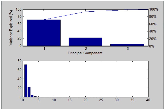
When the dimensionality of a data set is high, we use the PCA method to convert the set to one of lower dimensionality. PCA is a mathematical procedure that uses an orthogonal transformation to convert a set of observations of possibly correlated variables into a set of values of linearly uncorrelated variables
called principal components [7]. PCA is mathematically defined as an orthogonal linear transformation that transforms the data to a new coordinate system such that the greatest variance by any projection of the data comes to lie on the first coordinate (called the first principal component), the second greatest variance on the second coordinate, and so on.
Figure 1 shows, after PCA analysis, the main characteristic factors of the dataset, as well as their sum. It can be seen that the first three principal components of the sum of the contribution rate has reached 98%, so there are three main factors in the data set. Thus we can restrict ourselves to the analysis of only these three components.
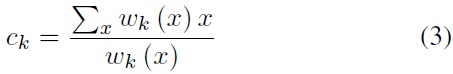
The FCM algorithm [8,9] attempts to partition a finite collection of n elements

where each element
which differs from the k-means objective function by the addition of the membership values
In fuzzy clustering, each point has a degree of belonging to clusters, as in fuzzy logic, rather than belonging completely to just one cluster. Thus, points on the edge of a cluster may be in a cluster to a lesser degree than points in the center of the cluster. An overview and comparison of different fuzzy clustering algorithms is available in [12].
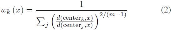
Any point x has a set of coefficients giving the degree of being in the
The degree of belonging,
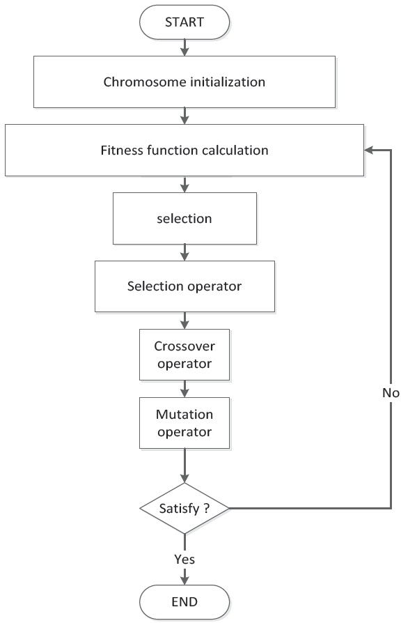
In the computer science field of artificial intelligence, a GA is a search heuristic that mimics the process of natural evolution [14-16]. This heuristic is routinely used to generate useful solutions to optimization and search problems. GAs belong to the larger class of evolutionary algorithms (EA), which generate solutions to optimization problems using techniques inspired by natural evolution, such as inheritance, mutation, selection, and crossover. The flowchart of a GA is shown in Figure 2.
Simple generational GA procedure:
1. Choose the initial population of individuals.
2. Evaluate the fitness of each individual in that population.
3. Repeat on this generation until termination (time limit, sufficient fitness achieved, etc.):
(1) Select the best-fit individuals for reproduction.
(2) Breed new individuals through crossover and mutation operations to give birth to offspring.
(3) Evaluate the individual fitness of new individuals.
(4) Replace least-fit population with new individuals.
3. Improve FCM Algorithm based on GA
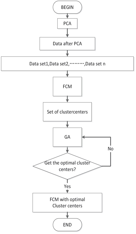
The flowchart of GA+FCM is shown in Figure 3. First, we input the KDDCUP1999 data. We then use PCA to process the data. The data pre-process method is shown in Section 2.2.
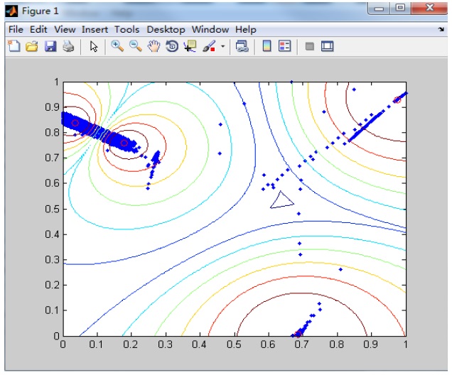
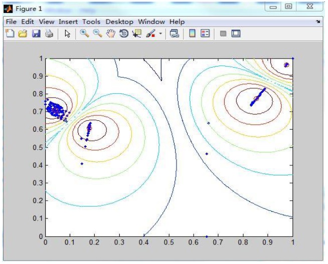
Next, the data is divided into many subsets of data. For example, in the data set used for Figure 4, there are 5000 data points, which are divided into 10 groups of equal size. We use the FCM clustering algorithm to determine the clustering center of each subset of data. We will show the GA processing in Section 2.4.
Figure 4 shows one group of 10 data sets. We use FCM to obtain its cluster centers, and the small red circles in the centers are the positions of cluster centers.
3.1.1 Code
An individual in a population is a cluster center [17]. To avoid the complexity of the encoding and to improve efficiency, we link the center of each group clustering. This helps to shorten chromosome length, and to improve the convergence speed and global optimum searching capability.
For example, the clustering center V= [
3.1.2 Fitness function
For the FCM algorithm, the optimal clustering results correspond to the minimum value of the objective function. Therefore, the individual fitness function can make use of the objective function of FCM algorithm for its definition.
The fitness function is:
where
3.1.3 Selection
Selection is the most important part of GA. In population evolutionary processes, the best individuals of the population are retained to avoid crossover and mutations, so that their desirable characteristics can be passed on to the next generation directly. The worst individuals do not participate in crossover, but they will have mutations with a larger probability than normal individuals. We then use the roulette method to choose the individuals, and we calculate the fitness function’s probability distribution for the populations. We choose individuals according to the probability distribution for crossover and mutation processing. In this way, we can improve the population’s average fitness performance. The selection probability function is defined via:
where
3.1.4 Crossover
We set (
3.1.5 Mutation
We set
<1> Set the cluster class equal to 4, the population to 40, the crossover rate to 0.3, the mutation rate to 0.5, and maximum number of iterations to 100.
<2> Calculate individual’s fitness through the fitness function.
<3> GA operations: selection, crossover, and mutation.
<4> Calculate the children’s fitness rate, and put them into their parents. Delete the individuals with low fitness rate.
<5> If the maximum iteration number is reached then return the individual with the largest fitness rate.
<6> End GA
We can get the optimal cluster centers through GA, and we use these cluster centers for the FCM algorithm’s initial value. We then use FCM to process the data. The result of using the optimal clustering with FCM as indicated in the above algorithm is shown in Figure 5 for a data set of 5000 points.
4. Experimental Result and Analysis
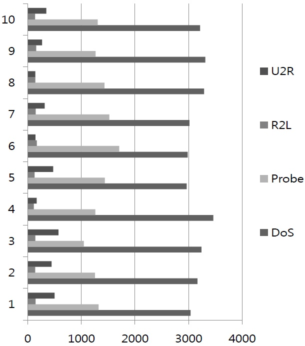
First, we extract 50000 data points from KDDCUP1999. We divided the data into 10 groups, as in Figure 6. The y-axis in the figure is data set number, and the x-axis in the figure is the size of the data used. The colors indicate attacks as the right side in Figure 6. The number of data points used is 5000 per group.
Using the algorithm from Section 3, we arrive at the conclusions in Table 1.
DR (detection rate) is the ratio of true intrusion instances detected by the system to the total number of intrusion instances in the data set.
OR (omission rate) is the ratio of the intrusion instances incorrectly identified by the system as non-intrusion instances to the total number of intrusion instances in the data set.
FR (false alarm) rate is ratio of the non-intrusion instances incorrectly identified by the system as intrusions to the total number of non-intrusion instances in the data set.
These rates are all defined with respect to the KDDCUP1999 data.
To facilitate analysis of the experimental results, we defined the function f(x)=DR(x)-OM(x)-FR(x) [19,20]. Our results are shown in Table 1.
The average DR shown in Table 1 is the average over the average detection rates of the 10 sets of data. Upon using the function f(x)=DR(x)-OM(x)-FR(x), we can determine the actual detection rate. The “FCM only” column gives the actual detection rate with only the FCM used to process the same data.
This paper uses a combination of a GA and the FCM method in intrusion detection. We solve the problems of the GA’s
[Table 1.] Experimental results
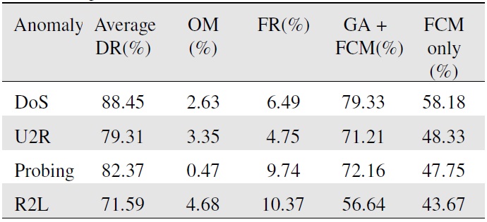
Experimental results
weakness for local search and the FCM’s weakness for global search. Consequently, we not only overcome the FCM algorithm’s sensitivity to the initial value and its tendency to yield local optimal solutions, but we can also utilize the GA’s primary strength of finding good global solutions. Through our experimental results, we find that the “GA+FCM” combined algorithm is better than the “FCM only” algorithm as measured by detection rate. However, the detection rate of our proposed method is not higher than that of other methods. Hence, more work is required to improve on this method. In future research, we will select other useful data mining methods to deal with these data and continue to reduce the redundancy in the data, and we will continue to learn about intrusion detection methods and find a more effective method to get a higher correct rate of intrusion detection.
No potential conflict of interest relevant to this article was reported.