Nowadays,the infrared imaging system is based on infrared focal-plane array (IRFPA) technology. However, the system has an inherent nonuniformity problem in that that the detectors in the array have different responses to the same input signal, causing the observed images to be degraded by fixed-pattern noise (FPN). In this case, many nonuniformity correction (NUC) techniques have been proposed to compensate for FPN. The NUC techniques include two classes that are reference-based and scene-based. Evidently, the scene-based methods are more attractive because the reference-based ones need to employ blackbody sources as uniform infrared targets while scene-based methods are conveniently updating the correction coefficients and avoiding scene interruptions.
So far, numerous scene-based nonuniformity correction (SBNUC) methods have been proposed. Assuming that each detector’s irradiance in the array has the same mean and variance, Y. M. Chiang and J. G. Harris proposed constant statistics (CS) methods [1,2]. References [2,3] aimed to increase convergence speed and reduce ghosting. S. N. Torres and M. M. Hayat presented a Kalman filter based method by a discrete-time Gauss-Markov process [4]. Another adaptive SBNUC technique is based on a neural network (NN) which is described in [5]. S. N. Torres, E. M. Vera improved the speed of the method by modifying the learning rate in the gain and offset parameter estimation process [6]. However, it is proved in reference [2] that the CS algorithm with appropriate coefficient has faster convergence rate and better performance than the LMS algorithm. Registration methods are proposed in [7,8]. But they all need complex registration algorithms and cannot work well when the nonuniformity is serious.
This paper puts forward a novel SBNUC algorithm called the med-CS method. This method is based on an improvement of the CS method. Due to the small influence of the median filter by an infrequent artifact and to the efficient capability for smoothing of impulsive-type noise, the proposed method utilizes the characteristics of median filter and applies it in the CS method to estimate the nonuniformity parameters. In the proposed algorithm, a temporal median is adopted combining with the Gaussian kernel. In this way, improvement in removal of ghosting artifacts and convergence speed can be achieved and the thorough analysis of effects on these two aspects is launched.
The remainder of the paper is organized as follows. In Section II the detector-level model and the readout amplifier model are given. Then the proposed algorithm is described and the superiority of the proposed algorithm is demonstrated. In Section III results obtained from simulated and real infrared data are presented. Finally, some conclusions are given in Section IV.
II. NONUNIFORMITY CORRECTION METHODS
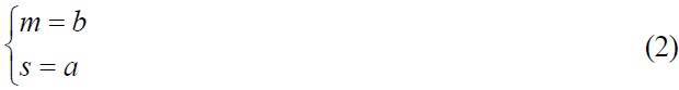
2.1. Observation Model and Conventional CS-NUC Method
The relationship between the observed infrared signal response and the real world is generally nonlinear. In literature [9],the output pixel value of each detector is modeled nonlinearly as a high order polynomial. To simplify the problem formulation for SBNUC, the linear approximation model is adopted which contains the first-order of the polynomial. Then the output of a single pixel is given by:

where,
Where,
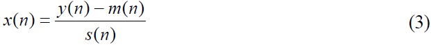
To estimate the gain and bias, the CS algorithm uses the mean of the measured output
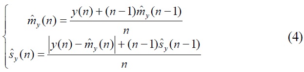
CS is improved to better estimate changes of gain and offset with a fixed-length rectangular and exponentially shaped window.
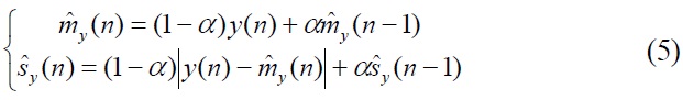
It can be seen from (5) that coefficient
2.2. The Proposed Med-CS NUC Method
The main drawback of the CS NUC method originates in the basic constraint that is related to the supposition that the scene is constantly moving. However, when the scene is not moving for a short while, the ghosting effect appears and the convergence rate will be affected. In this section, the proposed method takes a temporal median value with the Gaussian kernel and the ability of the method is analyzed.
2.2.1. Parameters estimation
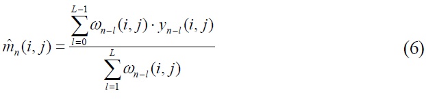
In the med-CS NUC method, the parameters for each pixel are calculated by computing weighted means and variances based on medians from the values with length of
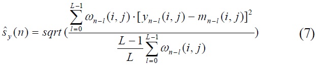
The weighted variance is expressed as:
The weights are computed from a Gaussian distribution centered at
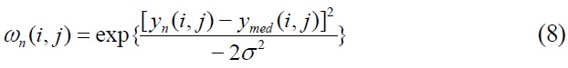
where

where the weights
2.2.2. Analysis of convergence
An assumption that the parameters of the nonuniformity are constant is employed, which means the offsets of sensors are considered to be fixed over time. According to the derivation in the literature [3] the mean-square error (

where
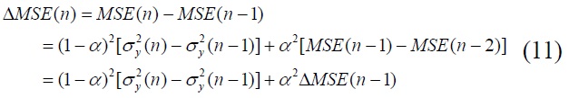
From (11), it can be seen that if
The CS method is based on the assumption that every pixel has the same distribution and the temporal mean and standard deviation of each pixel is constant over time and space. But the distribution tendency characteristic of each pixel over time has not been considered. The mean value that the CS method adopted is an appropriate measure of the central tendency. For instance the measurements of each pixel in a period of time has a Gaussian distribution. In fact, the temporal statistics of each pixel approximate mixture distributions rather than following a single distribution strictly. The mixture distribution contains more than two distributions. Regularly, there is more than three times difference among the deviations of the different distributions. Consequently, the deviation of the measurements cannot be constant over time and it will bring the problem according to (11) which was analyzed previously. To solve this problem a median value is utilized and proved to be effective by Monte Carlo simulation.
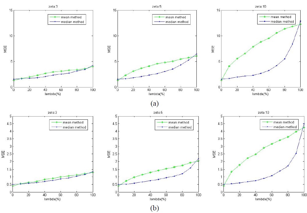
The median method, however, should have more perfect performance and this hypothesis is verified using Monte Carlo simulation. For this study, several groups of statistics were examined. Without loss of generality, an assumption is employed that the statistics consist of two Gaussian distributions with different deviations.

The simulation consists of 10,000 samples and each sample contains
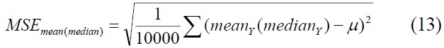
The result of the simulation is showed in Table 1,Table 2. Table 1 is generated by 10,000 samples with 50 values per sample, Table 2 is generated by 10,000 samples with 500 values per sample. The curves in Fig. 2(a) are drawn with the data in Table 1 and Fig. 2(b) is drawn with the data in Table 2.
The results display that the
Simultaneously, the coefficient
Finally, comparing Table 1 to Table 2 or comparing Fig. 2(a) to Fig. 2(b), it shows that the more sufficient the amount of data is, the maore superior the
From the above analysis the median method has a remarkable effect on eliminating interference of deviation variation. The median value is an accepted measure of the various tendencies
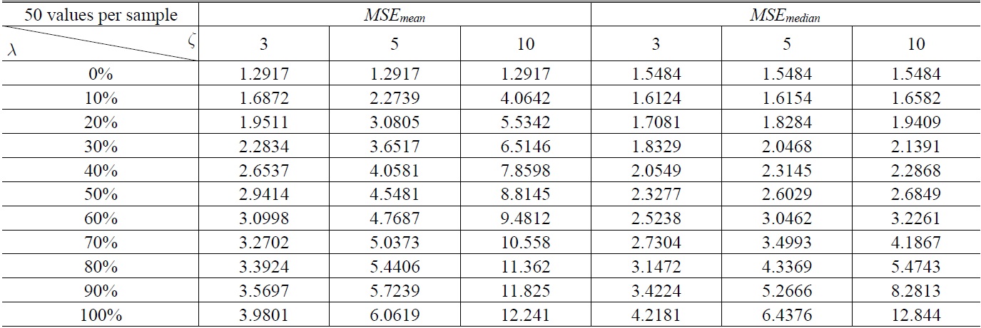
MSE of mean and median from Monte Carlo simulation for various samples (50 values per sample) from the different deviations observed distributions
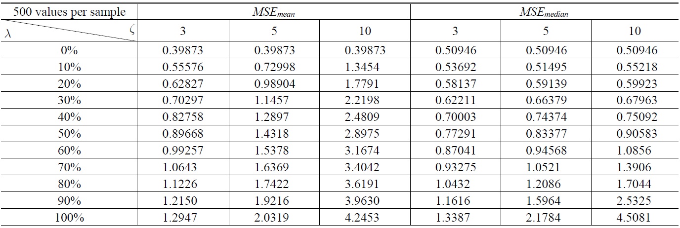
MSE of mean and median from Monte Carlo simulation for various samples (500 values per sample) from the different deviations observed distributions
of a group of values even when their distribution is non- Gaussian and the median method is valid even when applied to a small number of samples. Moreover the median method is less sensitive to the variation of sample distribution. Therefore, the med-CS using a temporal median is more robust and suitable to convergence than the conventional CS method.
In this section, the proposed med-CS method is applied to both simulated and real data to correct the nonuniformity compared with the various SBNUC algorithms and the method’s capability is verified.
3.1. Applications to Simulated Nonuniformity
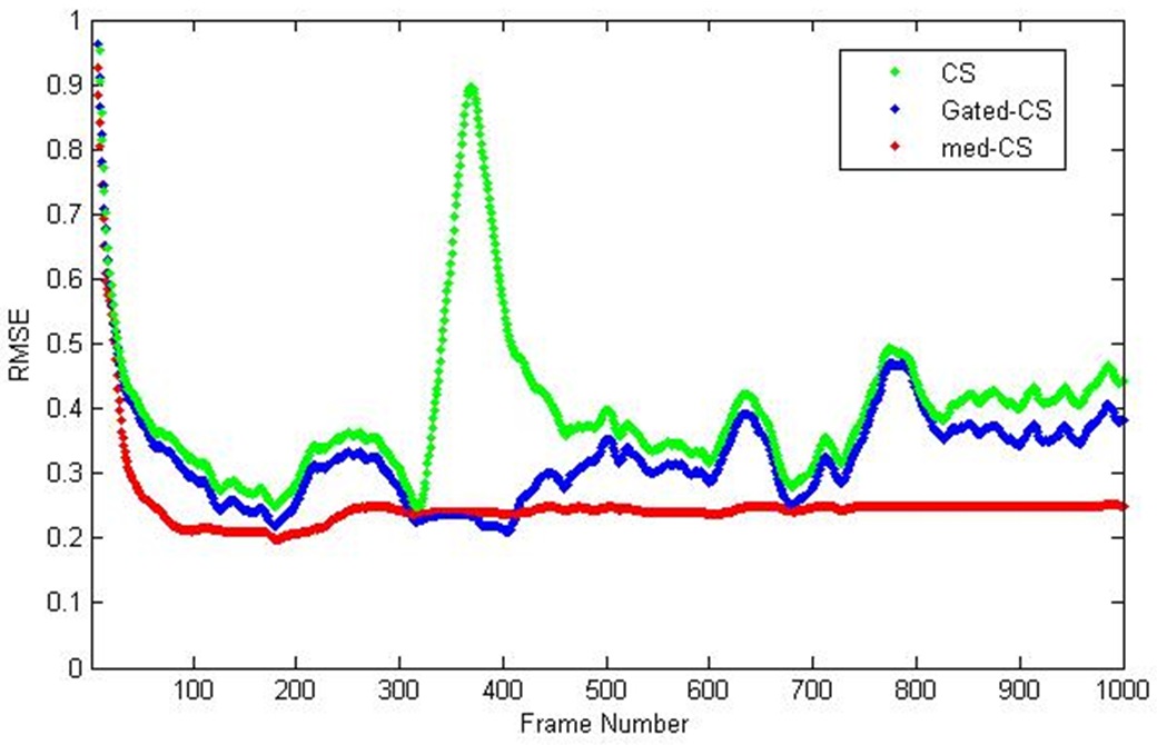
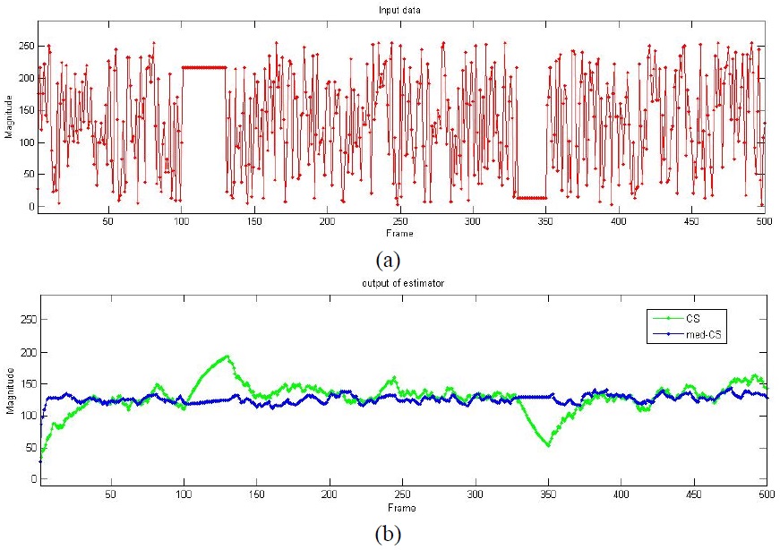
Several tests have been executed over an IR sequence of frames with simulated nonuniformity in this work. The deghosting capability has been demonstrated by visually comparing the frames obtained with the original CS method [1] and the improved CS method in [2]. Here, we call the method in [2] the gated-CS method because the algorithm sets a gated threshold to deghost.
As an evaluation criterion of correction performance, the Root Mean Square Error (
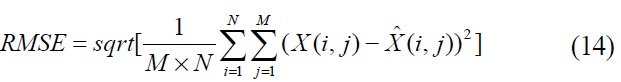
where

is the pixel’s value of the corrected frame and
The corrupted sequence with artificial nonuniformity is generated from a clear frame infrared video sequence with Simulated Nonuniformity added. The added FPN is composed of a synthetic gain with a unit-mean Gaussian distribution with standard deviation of 0.2, and a synthetic offset with a zero-mean Gaussian distribution with standard deviation of 15.
The CS method uses an exponential window parameter of
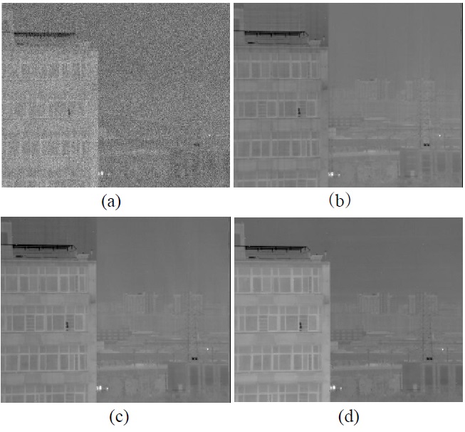
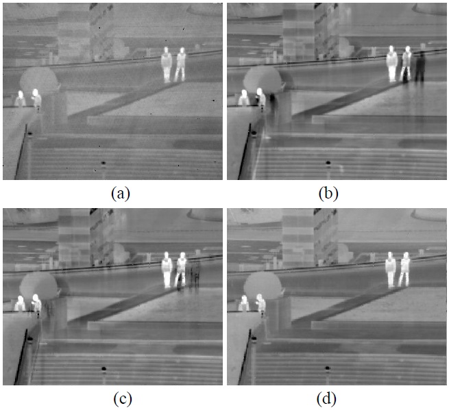
Figure 4 shows the images for the 780th frame. Fig. 4(a) shows the true clear infrared image corrupted with simulated nonuniformity. The NUC results of original CS method, gated-CS and med-CS algorithms are shown in Fig. 4(b) - (d). It is shown that the med-CS algorithm effectively generates much fewer ghosting artifacts than the other techniques.
3.2. Applications to Real Infrared Data
In this section, the original CS, gated-CS, and med-CS are applied to a noisy sequence collected by using a 320 × 256 HgCdTe IRFPA camera, operating in the 8 to 14
The coefficients used in the experiment are: the original CS method uses an exponential window parameter of
To indicate good correction performance or examine whether there is the presence of artifacts, a visual evaluation is performed by watching a video sequence. Fig. 5 shows the original image and the corrected images using the original CS, gated-CS, and med-CS algorithm of the 379th frame. It is very noticeable that the med-CS compensates the FPN and performs the best over the sequence. Besides, it effectively generates much fewer ghosting artifacts than the other techniques.
In this paper, based on the analysis of property of scene statistical distribution, a new NUC method called med-CS has been proposed, which adopts a temporal median filter combining with Gaussian kernel to estimate the NUC parameters. Taking advantage of the median filter’s characteristics properly, the proposed algorithm has the ability to improve the nonuniformity correction and eliminate ghosting artifacts efficiently. Experiments carried out with simulated nonuniformity and the real infrared data have shown that the proposed method offers the best performance compared with the conventional methods tested.