From Sep 2011 to Jun 2013, I was a visiting professor under the World Class University program of the Korean government, at the Korea Advanced Institute of Science and Technology (KAIST). My affiliation at KAIST was with the Division of Web Science and Technology (WebST), a newly established division with a primary mission to explore the relatively new but exciting area of Web science. In this invited paper, some of my research results contributing to that mission will be discussed. During my appointment with KAIST, I had retained my professorship at the Chinese University of Hong Kong, and worked at both institutions alternately during the development of these results, which therefore should be accredited to both institutions.

Existing search engines can reach only a small portion of the Internet. They crawl HTML pages interconnected with hyperlinks, which constitute one is known as the surface Web. An increasing number of organizations are bringing their data online, by allowing public users to query their back-end databases through context-dependent Web interfaces.

Data acquisition is performed by interacting with the interface at runtime, as opposed to following hyperlinks. As a result, the back-end databases cannot be effectively crawled by a search engine with current technology, and are usually referred to as hidden databases.

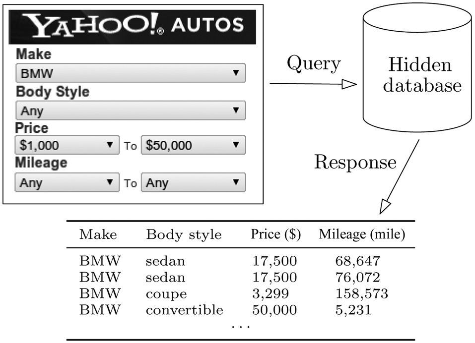
Consider Yahoo! Autos (autos.yahoo.com), a popular Website for the online trading of automobiles. A potential buyer specifies filtering criteria through a form, as illustrated in Fig. 1. The query is submitted to the system, which runs it against the back-end database, and returns the result to the user. What makes it non-trivial for a search engine to crawl the database is that setting all search criteria to ANY does not accomplish the task. The reason is that a system typically limits the number k of tuples returned (which is roughly 1000 for Yahoo! Autos), and that repeating the same query may not retrieve new tuples, with the same k tuples always being returned.

The ability of crawling a hidden database comes with

the appeal of enabling virtually any form of processing on the database’s content. The challenge, however, is clear: how to obtain all the tuples, given that the system limits the number of return tuples for each query. A naive solution is to issue a query for every single location in the data space (for example, in Fig. 1, the data space is the Cartesian product―while one may leverage knowledge of attribute dependencies (e.g., the fact that BMW does not sell trucks in the United States) to prune the data space into a subset of the Cartesian product, the subset is often still too large to enumerate―of the domains of MAKE, BODY STYLE, PRICE, and MILEAGE). However, the number of queries needed can clearly be prohibitive. This gives rise to an interesting problem, as defined in the next subsection, where the objective is to minimize the number of queries.

1) Problem Definitions

Consider that a data space

with d attributes A₁,..., A_d, each of which has a discrete domain. The domain of A_i denote by dom(A_i) for each i ∈ [1, d]. Then,

is the Cartesian product of dom(A₁), …, dom(A_d). We refer to each element of the Cartesian product as a point in

representing one possible combination of values of all dimensions.

A_i is a numeric attribute if there is a total ordering on dom(A_i). Otherwise, it is a categorical attribute. Our discussion distinguishes three types of

Numeric: all d attributes of

are numeric.

Categorical: all d attributes are categorical. In this case, we use Ui to represent the size of dom(Ai), which represents how many distinct values there are in dom(Ai).

Mixed: the first cat ∈ [1, d？1] attributes A1,…, Acat are categorical, whereas the other d ？ cat attributes are numeric. Similar to before, let Ui = |dom(Ai)| for each i ∈ [1, cat].

To facilitate presentation, we consider the domain of a numeric A_i to be the set of all integers, whereas that of a categorical A_i to be the set of integers from 1 to U_i. Keep in mind, however, that the ordering of these values is irrelevant to a categorical A_i.

Let D be the hidden database of a server with each element of D being a point in

To avoid ambiguity, we will always refer to elements of D as tuples. D is a bag (i.e., a multi-set), and it may contain identical tuples.

The server supports queries on D. As shown in Fig. 1, each query specifies a predicate on each attribute. Specifically, if A_i is numeric, the predicate is a range condition in the form of:

Ai ∈ [x, y]

where [x, y] is an interval in dom(A_i). For a categorical A_i, the predicate is:

Ai = x

where x is either a value in dom(A_i) or a wildcard ★. In particular, a predicate A_i = ★ means that A_i can be an arbitrary value in dom(A_i), as shown with capturing BODY STYLE = ANY in Fig. 1. If a hidden database server only allows single-value predicates on a numeric attribute (i.e., no range-condition support), then we can simply consider the attribute as categorical.

Given a query q, the bag of tuples in D qualifying all the predicates of q is denoted by q(D). The server does not necessarily return the entire q(D)―it does so only when q(D) is small. Formally, the response of the server is:

if |q(D)| ≤ k: the entire q(D) is returned. In this case, we say that q is resolved.

Otherwise: only k tuples―in practice, these are usually k tuples that have the highest priorities (e.g., according to a ranking function) among all the tuples qualifying the query―in q(D) are returned, together with a signal indicating that q(D) still has other tuples. In this case, we say that q overflows.

The value of k is a system parameter (e.g., k = 1,000 for Yahoo! Autos, as mentioned earlier). It is important to note that in the event that a query q overflows, repeatedly issuing the same q may always result in the same response from the server, and does not help to obtain the other tuples in q(D).

PROBLEM 1 (HIDDEN DATABASE CRAWLING). Retrieve the entire D while minimizing the number of queries.

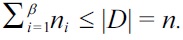
Recall that D is a bag, and it may have duplicate tuples. We require that no point in the data space

has more than k tuples in D. Otherwise, Problem 1 has no solution at all. To see this, consider the existence of k + 1 tuples t₁, ..., t_k+1 in D, all of which are equivalent to a point

Then, whenever p satisfies a query, the server can always choose to leave t_k+1 out of its response, making it impossible for any algorithm to extract the entire D. In Yahoo! Autos, this requirement essentially states that there cannot be k = 1,000 vehicles in the database with exactly the same values for all attributes―an assumption that is fairly realistic.

As mentioned in Problem 1, the cost of an algorithm is the number of queries issued. This metric is motivated by the fact that most systems have control over how many queries can be submitted by the same IP address within a period of time. Therefore, a crawler must minimize the number of queries to complete a task, in addition to minimizing the burden to the server.

We will use n to denote the number of tuples in D. It is clear that the number of queries needed to extract the entire D is at least n/k. Of course, this ideal cost may not always be possible. Hence, there are two central technical questions that need to be answered. The first, on the upper bound side, relates to how to solve Problem 1 by performing only a small number of queries even in the worst case. The second, on the lower bound side, concerns how many queries are compulsory for solving the problem in the worst case.

2) Our Results

We have concluded a systematic study of hidden database crawling as defined in Problem 1. At a high level, our first contribution is a set of algorithms that are both provably fast in the worst case, and efficient on practical data. Our second contribution is a set of lower-bound results establishing the hardness of the problem. These results explicitly clarify how the hardness is affected by the underlying factors, and thus reveal valuable insights into the characteristics of the problem. Furthermore, the lower bounds also prove that our algorithms are already optimal asymptotically, and cannot be improved by more than a constant factor.

Our first main result is:

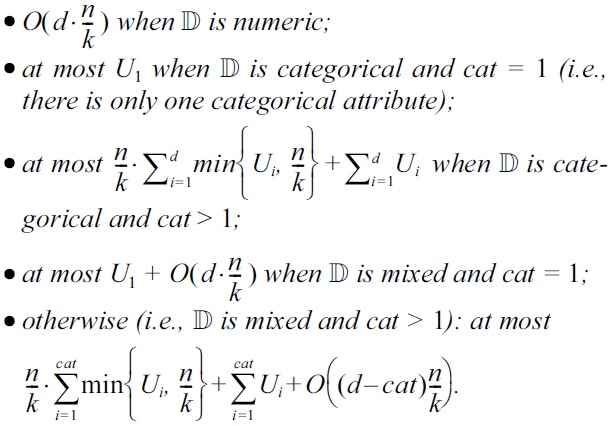
THEOREM 1. There is an algorithm for solving Problem 1 whose cost is:

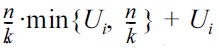
The above can be conveniently understood as follows: our algorithm pays an additive cost of O(n/k) for each numeric attribute A_i, whereas it pays

for each categorical A_i. The only exception is when cat = 1: in this scenario, we pay merely U₁ for the (only) categorical attribute A₁. The cost of each numeric attribute is irrelevant to its domain size.

Our second main result complements the preceding one:

THEOREM 2. None of the results in Theorem 1 can be improved by more than a constant factor in the worst case.

Besides establishing the optimality of our upper bounds in Theorem 1, Theorem 2 has its own interesting implications. First, it indicates the unfortunate fact that for all types of

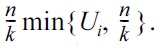
the best achievable query time in the worst case is much higher than the ideal cost of n/k. Nevertheless, Theorem 1 suggests that we can achieve this cost asymptotically when d is a constant and all attributes are numeric. Second, as the number cat of categorical attributes increases from 1 to 2, the discrepancy of the time complexities in Theorem 1 is not an artifact, but rather, it is due to an inherent leap in the hardness of the problem (which is true regardless of the number of numeric attributes). That is, while we pay only O(U₁) extra queries for the (sole) categorical attribute when cat = 1, as cat grows to 2 and beyond, the cost paid by any algorithm for each categorical A_i has an extra term of

Given that the term is multiplicative, this finding implies (perhaps surprisingly) that, in the worst case, it may be infeasible to crawl a hidden database with a large size n, and at least 2 categorical attributes such that at least one of them has a large domain.

In this paper, we prove Theorems 1 and 2 only for the case where

is numeric. The rest of the proof is available elsewhere [1].

We are in an era of information explosion, where industry, academia, and governments are accumulating data at an unprecedentedly high speed. This brings forward the urgent need for fast computation over colossal datasets whose sizes can reach the order of terabytes or higher. In recent years, the database community has responded to this challenge by building massive parallel computing platforms which use hundreds or even thousands of commodity machines. The most notable platform thus far is MapReduce, which has attracted a significant amount of attention in research.

Since its invention [2], MapReduce has gone through years of improvement into a mature paradigm. At a high level, a MapReduce system involves a number of sharenothing machines which communicate only by sending messages over the network. A MapReduce algorithm instructs these machines to perform a computational task collaboratively. Initially, the input dataset is distributed across the machines, typically in a non-replicate manner, with each object on one machine. The algorithm executes in rounds (sometimes also called jobs in the literature), each having three phases: map, shuffle, and reduce. The first two enable the machines to exchange data. In the map phase, each machine prepares the information to be delivered to other machines, while the shuffle phase takes care of the actual data transfer. No network communication occurs in the reduce phase, where each machine performs calculation with its local storage. The current round finishes after the reduce phase. If the computational task has not completed, another round starts.

As with traditional parallel computing, a MapReduce system aims to achieve a high degree of load balancing, as well as the minimization of space, CPU, I/O, and network costs at each individual machine. Although these principles have guided the design of MapReduce algorithms, previous practices have mostly been on a besteffort basis, paying relatively less attention to enforcing serious constraints on different performance metrics. Our work aims to remedy the situation by studying algorithms that promise outstanding efficiency in multiple aspects simultaneously.

1) Minimal MapReduce Algorithms

Let S be the set of input objects for the underlying problem. Let n be the problem cardinality, which is the number of objects in S, and t be the number of machines used in the system. Define m = n/t, where m is the number of objects per machine when S is evenly distributed across the machines. Consider an algorithm for solving a problem on S. We say that the algorithm is minimal if it has all of the following properties:

Minimum footprint: at all times, each machine uses only O(m) space of storage.

Bounded net-traffic: in each round, every machine sends and receives at most O(m) words of information over the network.

Constant round: the algorithm must terminate after a constant number of rounds.

Optimal computation: every machine performs only O(Tseq/t) amount of computation in total (i.e., summing over all rounds), where Tseq is the time needed to solve the same problem on a single sequential machine. The algorithm should achieve a speedup of t by using t machines in parallel.

It is fairly intuitive why minimal algorithms are appealing. First, a minimum footprint ensures that each machine keeps O(1/t) of the dataset S at any moment. This effectively prevents partition skew, where some machines are forced to handle considerably more than m objects, as is a major cause of inefficiency in MapReduce [3].

Second, bounded net-traffic guarantees that the shuffle phase of each round transfers at most O(m·t) = O(n) words of network traffic overall. The duration of the phase equals roughly the time for a machine to send and receive O(m) words, because the data transfers between different machines are in parallel. Furthermore, this property is also useful when one wants to make an algorithm stateless for the purpose of fault tolerance.

The third property constant round is not new, as it has been the goal of many previous MapReduce algorithms. Importantly, this and the previous properties imply that there can be only O(n) words of network traffic during the entire algorithm. Finally, optimal computation echoes the very original motivation of MapReduce to accomplish a computational task t times faster than leveraging only one machine.

2) Our Results

The core of this work comprises a neat minimal algorithm for:

Sorting. The input is a set S of n objects drawn from an ordered domain. When the algorithm terminates, all the objects must have been distributed across the t machines in a sorted fashion. That is, we can order the machines from 1 to t such that all objects in machine i precede those in machine j for all 1 ≤ i ≤ j ≤ t.

Sorting can be settled in O(n log n) time on a sequential computer. There has been progress in developing MapReduce algorithms for this important operation. The state of the art is TeraSort [4], which won Jim Gray’s benchmark contest in 2009. TeraSort comes close to being minimal when a crucial parameter is set appropriately. As will be made clear later, the algorithm requires manual tuning of the parameter, an improper choice of which can incur severe performance penalties.

Our work was initialized by an attempt to justify theoretically why TeraSort often achieves excellent sorting time with only 2 rounds. In the first round, the algorithm extracts a random sample set S_samp of the input S, and then picks t ？ 1 sampled objects as the boundary objects. Conceptually, these boundary objects divide S into t segments. In the second round, each of the t machines acquires all the objects in a distinct segment, and sorts them. The size of S_samp is the key to efficiency. If S_samp is too small, the boundary objects may be insufficiently scattered, which can cause partition skew in the second round. Conversely, an over-sized S_samp entails expensive sampling overhead. In the standard implementation of TeraSort, the sample size is left as a parameter, although it always seems to admit a good choice that gives outstanding performance [4].

We provide a rigorous explanation of the above phenomenon. Our theoretical analysis clarifies how to set the size of S_samp to guarantee the minimality of TeraSort. In the meantime, we also remedy a conceptual drawback of TeraSort. Strictly speaking, this algorithm does not fit in the MapReduce framework, because it requires that, besides network messages, the machines should be able to communicate by reading/writing a common distributed file. Once this is disabled, the algorithm requires one more round. We present an elegant fix so that the algorithm still terminates in 2 rounds even by strictly adhering to MapReduce. Our findings with TeraSort have immediate practical significance, given the essential role of sorting in a large number of MapReduce programs.

It is worth noting that a minimal algorithm for sorting leads to minimal algorithms for several fundamental database problems, including ranking, group-by, semi-join, and skyline [5].

This section explains how to solve Problem 1 when the data space

is numeric. In Section II-A, we first define some atomic operators, and present an algorithm that is intuitive, but has no attractive performance bounds. Then, in Sections II-B and II-C, we present another algorithm, which achieves the optimal performance, as proven in Section II-D.

Recall that in a numeric

the predicate of a query q on each attribute is a range condition. Thus, q can be regarded as a d-dimensional (axis-parallel) rectangle, such that its result q(D) consists of the tuples of D covered by that rectangle. If the predicate of q on attribute A_i (i ∈ [1, d]) is A_i ∈ [x₁, x₂], we say that [x₁, x₂] is the extent of the rectangle of q along A_i. Henceforth, we may use the symbol q to refer to its rectangle also, when no ambiguity can be caused. Clearly, settling Problem 1 is equivalent to determining the entire q(D) where q is the rectangle covering the whole

Split. A fundamental idea to extract all the tuples in q(D) is to refine q into a set S of smaller rectangles, such that each rectangle q' ∈ S can be resolved (i.e., q'(D) has at most k tuples). Note that this always happens as long as rectangle q' is sufficiently small. In an the extreme case, when q' has degenerated into a point in

the query q' is definitely resolved (otherwise, there would be at least k + 1 tuples of D at this point). Therefore, a basic operation in our algorithms for Problem 1 is split.

Given a rectangle q, we may perform two types of splitting, depending on how many rectangles q is divided into:

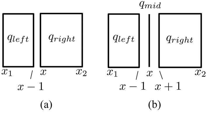
1) 2-way split: Let [x1, x2] be the extent of q on Ai (for some i ∈ [1, d]). A 2-way split at a value x ∈ [x1, x2] partitions q into rectangles qleft and qright, by dividing the Ai-extent of q at x. Formally, on any attribute other than Ai, qleft and qright have the same extents as q. Along Ai, however, the extent qleft is [x1, x ？ 1], whereas that of qright is [x, x2]. Fig. 2a illustrates the

idea by splitting on the horizontal attribute.

2) 3-way split: Let [x1, x2] be defined as above. A 3-way split at a value x ∈ [x1, x2] partitions q into rectangles qleft, qmid, and qright as follows. On any attribute other than Ai, they have the same extent as q. Along Ai, however, the extent of qleft is [x1, x ？ 1], that of qmid is [x, x], and that of qright is [x + 1, x2] (Fig. 2b).

In the sequel, a 2-way split will be abbreviated simply as a split. No confusion can arise as long as we always mention 3-way as referring to a 3-way split. The extent of a query q on an attribute A_i can become so short that it covers only a single value, in which case we say that A_i is exhausted on q. For instance, the horizontal attribute is exhausted on q_mid in Fig. 2b. It is easy to see that there is always a non-exhausted attribute on q unless q has degenerated into a point.

Binary-shrink. Next, we describe a straightforward algorithm for solving Problem 1, which will serve as the baseline approach for comparison. This algorithm, named binary-shrink, repeatedly performs 2-way splits until a query is resolved. Specifically, given a rectangle q, binary-shrink runs the rectangle (by submitting its corresponding query to the server) and finishes if q is resolved. Otherwise, the algorithm splits q on an attribute A_i that has not been exhausted, by cutting the extent [x₁, x₂] of q along A_i into equally long intervals (i.e., the split is performed at x = ？(x₁+ x₂)/2？). Let q_left, q_right be the queries produced by the split. The algorithm then recurses on q_left and q_right.

It is clear that the cost of binary-shrink (i.e., the number of queries issued) depends on the domain sizes of the numeric attributes of

which can be unbounded. In the following subsections, we will improve this algorithm to optimality.

Before giving our ultimate algorithm for settling Problem 1 with any dimensionality d, in this subsection, we first explain how it works for d = 1. This will clarify the rationale behind the algorithm’s efficiency, and facilitate our analysis for a general d. It is worth mentioning that the presence of only one attribute removes the need to specify the split dimension in describing a split.

Rank-shrink. Our algorithm rank-shrink differs from binary-shrink in two ways. First, when performing a 2-way split, instead of cutting the extent of a query q in half, we aim at ensuring that at least k/4 tuples fall in each of the rectangles generated by the split. Such a split, however, may not always be possible, which can happen if many tuples are identical to each other. Hence, the second difference that rank-shrink makes is to perform a 3-way split in such a scenario, which gives birth to a query (among the 3 created) that can be immediately resolved.

Formally, given a query q, the algorithm eventually returns q(D). It starts by issuing q to the server, which returns a bag R of tuples. If q is resolved, the algorithm terminates by reporting R. Otherwise (i.e., in the event that q overflows), we sort the tuples of R in ascending order, breaking ties arbitrarily. Let o be the (k/2)-th tuple in the sorted order, with its A₁-value being x. Now, we count the number c of tuples in R identical to o (i.e., R has c tuples with A₁-value x), and proceed as follows:

1) Case 1: c ≤ k/4. Split q at x into qleft and qright, each of which must contain at least k/4 tuples in R. To see this for qleft (symmetric reasoning applies to qright), note there are at least k/2 ？ c ≥ k/4 tuples of R strictly smaller than x, all of which fall in qleft. The case for qright follows in analogy.

2) Case 2: c > k/4. Perform a 3-way split on q at x. Let qleft, qmid, and qright be the resulting rectangles (note that the ordering among them matters; see Section II-B). Observe that qmid has degenerated into point x, and therefore, can immediately be resolved. As a technical remark, in Case 2, x might be the lower (resp. upper) bound―x cannot be both because otherwise q would be a point and therefore could not have overflowed―on the extent of q. If this happens, we simply discard qleft (or qright) as it would have a meaningless extent.

In either case, we are left with at most two queries (i.e., q_left and q_right) to further process. The algorithm handles each of them recursively in the same manner.

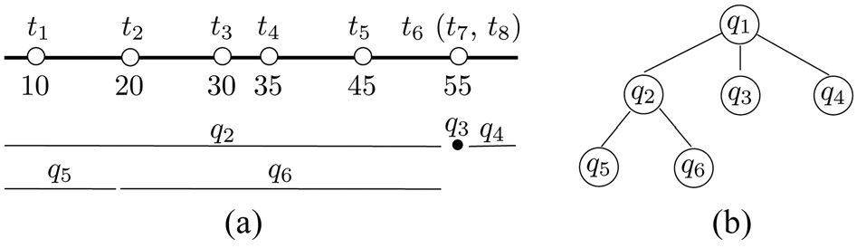
Example. We use the dataset D in Fig. 3a to demonstrate the algorithm. Let k = 4. The first query is q₁ = (？∞, ∞). Suppose that the server responds by returning R₁ = {t₄, t₆, t₇, t₈} and a signal that q₁ overflows. The (k/2) = 2nd smallest tuple in R₁ is t₆ (after random tie breaking), whose value is x = 55. As R₁ has c = 3 tuples with value 55 and c > k/4 = 1, we perform a 3-way split on q₁ at 55, generating q₂ = (？∞, 54], q₃ = [55, 55], and q₄ = [56, ∞). As q₃ has degenerated into a point, it is resolved immediately, fetching t₆, t₇, and t₈. These tuples have already been extracted before, but this time they come with an extra fact that no more tuple can exist at point 55.

Consider q₂. Suppose that the server’s response is R₂ = {t₁, t₂, t₄, t₅}, plus an overflow signal. Hence, x = 20 and c = 1. Thus, a 2-way split on q₂ at 20 creates q₅ = (？∞, 19]

and q₆ = [20, 54]. Queries q₄, q₅, and q₆ are all resolved.

Analysis. The lemma below bounds the cost of rank-shrink.

LEMMA 1. When d = 1, rank-shrink requires O(n/k) queries.

Proof. The main tool used by our proof is a recursion tree T that captures the spawning relationships of the queries performed by rank-shrink. Specifically, each node of T represents a query. Node u is the parent of node u' if query u' is created by a 2-way or 3-way split of query u. Each internal node thus has 2 or 3 child nodes. Fig. 3b shows the recursion tree for the queries performed in our earlier example on Fig. 3a.

We focus on bounding the number of leaves in T because it dominates the number of internal nodes. Observe that each leaf v corresponds to a disjoint interval in dom(A₁), due to the way splits are carried out. There are three types of v:

Type-1: the query represented by v is immediately resolved in a 3-way split (i.e., qmid in Case 2). The interval of v contains at least k/4 identical tuples in D.

Type-2: query v is not type-1, but also covers at least k/4 tuples in D.

Type-3: query v covers less than k/4 tuples in D.

For example, among the leaf nodes in Fig. 3, q₃ is of type-1, q₅ and q₆ are of type-2, and q₄ is of type-3.

As the intervals of various leaves cover disjoint bags of tuples, the number of type-1 and type-2 leaves is at

Each leaf of type-3 must have a sibling in T that is a type-2 leaf (in Fig. 3, such a sibling of q₄ is q₃). In contrast, a type-2 leaf has at most 2 siblings. It thus follows that there are at most twice as many type-3 leaves as type-2, i.e., the number of type-3 leaves is no more than 8n/k. This completes the proof.

This analysis implies that quite loosely, T has no more than 4n/k + 8n/k = 12n/k leaves. Thus, there cannot be more than this number of internal nodes in T. □

We are now ready to extend rank-shrink to handle any d > 1. In addition to the ideas exhibited in the preceding subsection, we also apply an inductive approach, which involves converting the d-dimensional problem to several (d ？ 1)-dimensional ones. Our discussion below assumes that the (d ？ 1)-dimensional problem has already been settled by rank-shrink.

Given a query q, the algorithm (as in 1d) sets out to solicit the server’s response R, and finishes if q is resolved. Otherwise, it examines whether A₁ is exhausted in q, and whether the extent of q on A₁ has only 1 value x in dom(A₁). If so, we can then focus on attributes A₂, ..., A_d. This is a (d ？ 1)-dimensional version of Problem 1, in the (d ？ 1)-dimensional subspace covered by the extents of q on A₂, ..., A_d, eliminating A₁ by fixing it to x. Hence, we invoke rank-shrink to solve it.

Consider that A₁ is not exhausted on q. Similar to the 1d algorithm, we will split q such that either every resulting rectangle covers at least k/4 tuples in R, or one of them can be immediately solved as a (d ？ 1)-dimensional problem. The splitting proceeds exactly as described in Cases 1 and 2 of Section II. The only difference is that the rectangle q_mid in Case is not a point, but instead, a rectangle on which A₁ has been exhausted. Hence, q_mid is processed as a (d ？ 1)-dimensional problem with rank-shrink.

As with the 1d case, the algorithm recurses on q_left and q_right (provided that they have not been discarded for having a meaningless extent on A₁).

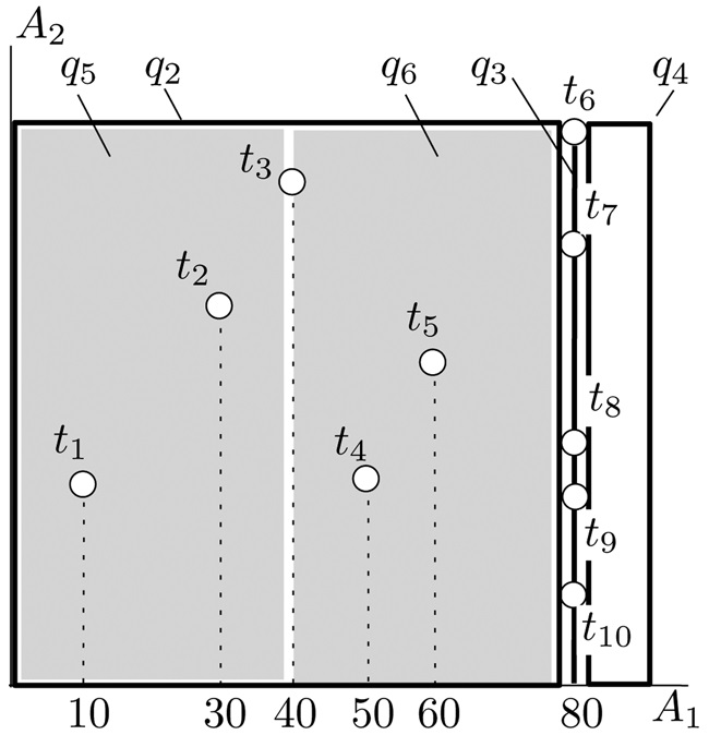
Example. We demonstrate the algorithm using the 2d dataset in Fig. 4, where D has 10 tuples t₁, ..., t₁₀. Let k = 4. The first query q₁ issued covers the entire data space. Suppose that the server responds with R₁ = {t₄, t₇, t₈, t₉} and an overflow signal. We split q₁ 3-ways at A₁ = 80 into q₂, q₃, and q₄, whose rectangles can be found in Fig. 4. The A₁-extents of q₂, q₃, and q₄ are (？∞, 79], [80, 80], and [81, ∞), respectively, while their A₂-extents are all (？∞, ∞). Note that A₁ is exhausted on q₂; alternatively, we can see that q₂ is equivalent to a 1d query on the vertical line A₁ = 80. Hence, q₂ is recursively settled by our 1d algorithm (requiring 3 queries, which can be verified easily).

Suppose that the server’s response to q₂ is R₂ = {t₂, t₃, t₄, t₅} and an overflow signal. Accordingly, q₂ is split into q₅ and q₆ at A₁ = 40, whose rectangles are also shown in Fig. 4. Finally, q₄, q₅, and q₆ are all resolved.

Analysis. We have the lemma below for general d:

LEMMA 2. Rank-shrink performs O(dn/k) queries.

Proof. The case d = 1 has been proven in Lemma 1.

Next, assuming that rank-shrink issues at most α(d ？ 1)n/k queries for solving a (d ？ 1)-dimensional problem with n tuples (where α is a positive constant), we will show that the cost is at most αdn/k for dimensionality d.

Again, our argument leverages a recursion tree T. As before, each node of T is a query, such that node u parents node u', if query u' was created from splitting u. We make a query v a leaf of T as soon as one of the following occurs:

v is resolved. We associate v with a weight set to 1.

A1 is exhausted on rectangle v. Recall that such a query is solved as a (d ？ 1)-dimensional problem. We associate v with a weight, equal to the cost for rank-shrink for that problem.

For our earlier example in Fig. 4, the recursion tree T happens to be the same as the one in Fig. 3b. The difference is that each leaf has a weight. Specifically, the weight of q₃ is 3 (i.e., the cost of solving the 1d query at the vertical line A₁ = 80 in Fig. 4), and the weights of the other leaves are 1.

Therefore, the total cost of rank-shrink on the d-dimensional problem is equal to the total number of internal nodes in T, plus the total weight of all the leaves.

As the A₁-extents of the leaves’ rectangles have no overlap, their rectangles cover disjoint tuples. Let us classify the leaves into type-1, -2, and -3, as in the proof of Lemma 1, by adapting the definition of type-1 in a straightforward fashion: v is of this type if it is the middle node q_mid from a 3-way split. Each type-leaf has weight 1 (as its corresponding query must be resolved). As proved in Lemma 1, the number of them is no more than 8n/k.

Let v₁,..., v_β be all the type-1 and type-2 nodes (i.e., suppose the number of them is β). Assume that node v_i contains n_i tuples of D. It holds that

The weight of v_i, by our inductive assumption, is at most α(d ？ 1)n_i/k. Hence, the total weight of all the type-1 and type-2 nodes does not exceed α(d ？ 1)n/k.

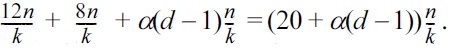
The same argument in the proof of Lemma 1 shows that T has less than 12n/k internal nodes. Thus, summarizing the above analysis, the cost of d-dimensional rank-shrink is no more than:

To complete our inductive proof, we want

to be bounded from above by αdn/k. This is true for any α ≥ 20. □

Remark. This concludes the proof of the first bullet of Theorem 1. When d is a fixed value (as is true in practice), the time complexity in Lemma 2 becomes O(n/k), asymptotically matching the trivial lower bound n/k. A natural question at this point of whether there is an algorithm that can still guarantee cost O(n/k) if d is not constant, Next, we will show that this is impossible.

The objective of this subsection is to establish:

THEOREM 3. Let k, d, and m be arbitrary positive integers such that d ≤ k. There is a dataset D (in a numeric data space) with n = m(k + d) tuples such that any algorithm must use at least dm queries to solve Problem 1 on D.

It is therefore impossible to improve our algorithm rank-shrink (see Lemma 2) by more than a constant factor in the worst case, as shown below:

COROLLARY 1. In a numeric data space, no algorithm can guarantee solving Problem 1 with o(dn/k) queries.

Proof. If there existed such an algorithm, let us use it on the inputs in Theorem 3. The cost is o(dn/k) = o(dm(k+d)/k) which, due to d ≤ k, is o(dm), causing a contradiction. □

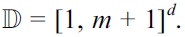
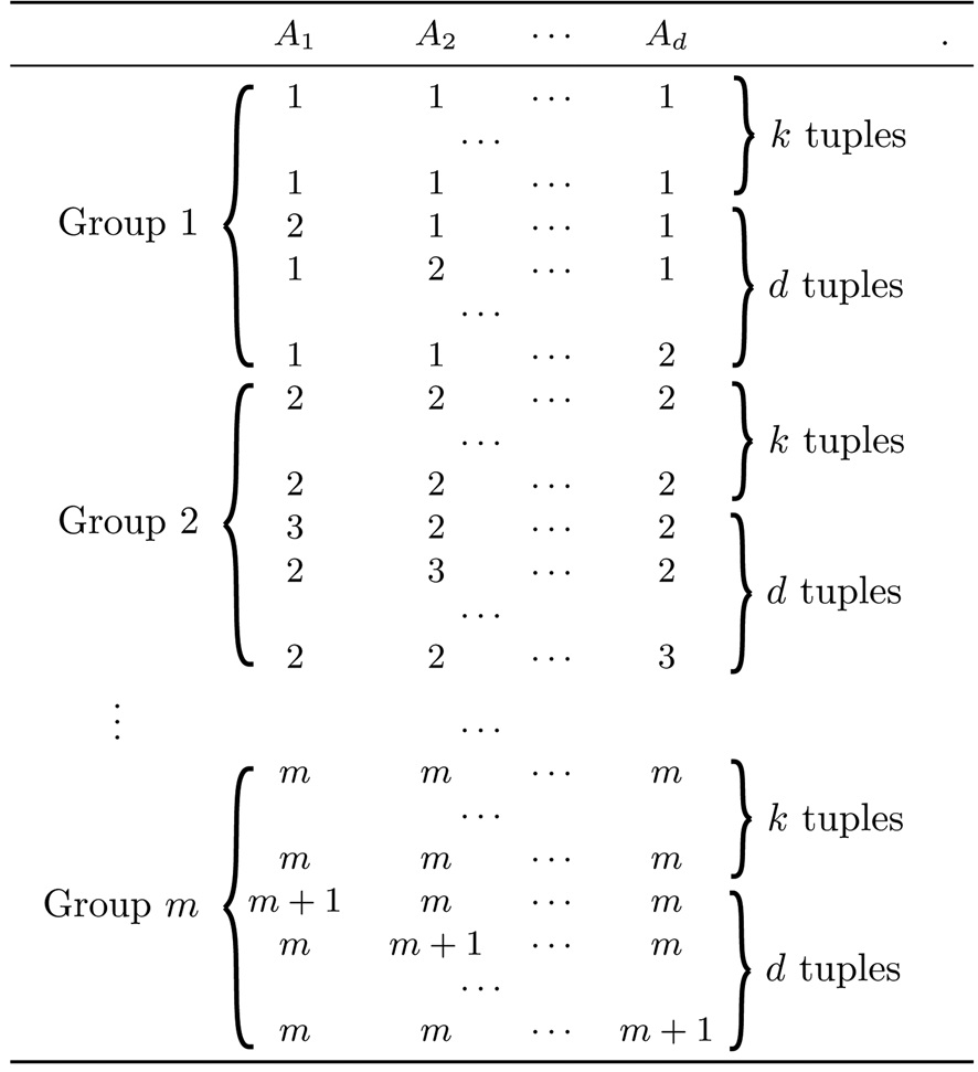
We now proceed to prove Theorem 3 using a hard dataset D, as illustrated in Fig. 5. The domain of each attribute is the set of integers from 1 to m +1, or

D has m groups of d + k tuples. Specifically, the i-th group (1 ≤ i ≤ m) has k tuples at the point (i, ..., i), taking value i on all attributes. We call them diagonal tuples. Furthermore, for each j ∈ [1, d], group i also has a tuple that takes value i + 1 on attribute A_j, and i on all other attributes. Such a tuple is referred to as a non-diagonal

tuple. Overall, D has km diagonal and dm non-diagonal tuples.

Let S be the set of dm points in

that are equivalent to the dm non-diagonal tuples in D, respectively (i.e., each point in S corresponds to a distinct non-diagonal tuple). As explained in Section II-A, each query can be regarded as an axis-parallel rectangle in

With this correspondence in mind, we observe the following for any algorithm that correctly solves Problem 1 on D.

LEMMA 3. When the algorithm terminates, each point in S must be covered by a distinct resolved query already performed.

Proof. Every point p ∈ S must be covered by a resolved query. Otherwise, p is either never covered by any query, or covered by only overflowing queries. In the former case, the tuple of D at p could not have been retrieved, whereas in the latter, the algorithm could not rule out the possibility that D had more than one tuple at p. In neither case could the algorithm have terminated.

Next, we show that no resolved query q covers more than one point in S. Otherwise, assume that q contains p₁ and p₂ in S, in which case q fully encloses the minimum bounding rectangle, denoted as r, of p₁ and p₂. Without loss of generality, suppose that p₁ (p_j) is from group i (j) such that i ≤ j. If i = j, then r contains the point (i, ..., i), in which case at least k + 2 tuples satisfy q (i.e., p₁, p₂, and the k diagonal tuples from group i). Alternatively, consider i < j. In this scenario, the coordinate of p₁ is at most i + 1 ≤ j on all attributes, while the coordinate of p₂ is at least j on all attributes. Thus, r contains the point (j, ..., j), causing at least k + 2 tuples to satisfy q (i.e., p₁, p₂, and the k diagonal tuples from group j). Therefore, q must overflow in any case, which is a contradiction. □

The lemma indicates that at least |S| = dm queries must be performed, which validates Theorem 3.

As explained earlier, a MapReduce algorithm proceeds in rounds, where each round has three phases: map, shuffle, and reduce. As all machines execute a program in the same way, next we focus on one specific machine M.

Map. In this phase, M generates a list of key-value pairs (k, v) from its local storage. While the key k is usually numeric, the value v can contain arbitrary information. The pair (k, v) will be transmitted to another machine in the shuffle phase, such that the recipient machine is determined solely by k, as will be clarified shortly.

Shuffle. Let L be the list of key-value pairs that all the machines produced in the map phase. The shuffle phase distributes L across the machines adhering to the constraint that pairs with the same key must be delivered to the same machine. That is, if (k, v₁), (k, v₂),..., (k, v_x) are the pairs in L having a common key k, all of them will arrive at an identical machine.

Reduce. M incorporates the key-value pairs received from the previous phase into its local storage. Then, it carries out whatever processing is needed on its local data. After all machines have completed the reduce phase, the current round terminates.

Discussion. It is clear that the machines communicate only in the shuffle phase, whereas in the other phases each machine executes the algorithm sequentially, focusing on its own storage. Overall, parallel computing happens mainly in the reduce phase. The major role of the map and shuffle phases is to swap data among the machines, so that computation can take place on different combinations of objects.

Simplified view of our algorithms. Let us number the t machines of the MapReduce system arbitrarily from 1 to t. In the map phase, all our algorithms will adopt the convention that M generates a key-value pair (k, v) if and only if it wants to send v to machine k. In other words, the key field is explicitly the ID of the recipient machine.

This convention admits a conceptually simpler modeling. In describing our algorithms, we will combine the map and shuffle phases into one called map-shuffle. In the map-shuffle phase, M delivers v to machine k, which means that M creates (k, v) in the map phase, which is then transmitted to machine k in the shuffle phase. The equivalence also explains why the simplification is only at the logical level, while physically, all our algorithms are still implemented in the standard MapReduce paradigm.

Statelessness for fault tolerance. Some MapReduce implementations (e.g., Hadoop) require that at the end of a round, each machine should send all the data in its storage to a distributed file system (DFS), which, in our context, can be understood as a “disk in the cloud” that guarantees consistent storage (i.e., it never fails). The objective is to improve the system’s robustness in the scenario where a machine collapses during the algorithm’s execution. In such a case, the system can replace this machine with another one, ask the new machine to load the storage of the old machine at the end of the previous round, and re-do the current round (where the machine failure occurred). Such a system is called stateless, because intuitively, no machine is responsible for remembering any state of the algorithm [6].

The four minimality conditions defined in Section I ensure efficient enforcement of statelessness. In particular, a minimum footprint guarantees that at each round, every machine sends O(m) words to the DFS, which is still consistent with bounded traffic.

In the sorting problem, the input is a set S of n objects from an ordered domain. For simplicity, we assume that objects are real values, because our discussion easily generalizes to other ordered domains. Let M₁,..., M_t denote the machines in the MapReduce system. Initially, S is distributed across these machines, each storing O(m) objects, where m = n/t. At the end of sorting, all objects in M_i must precede those in M_j for any 1 ≤ i < j ≤ t.

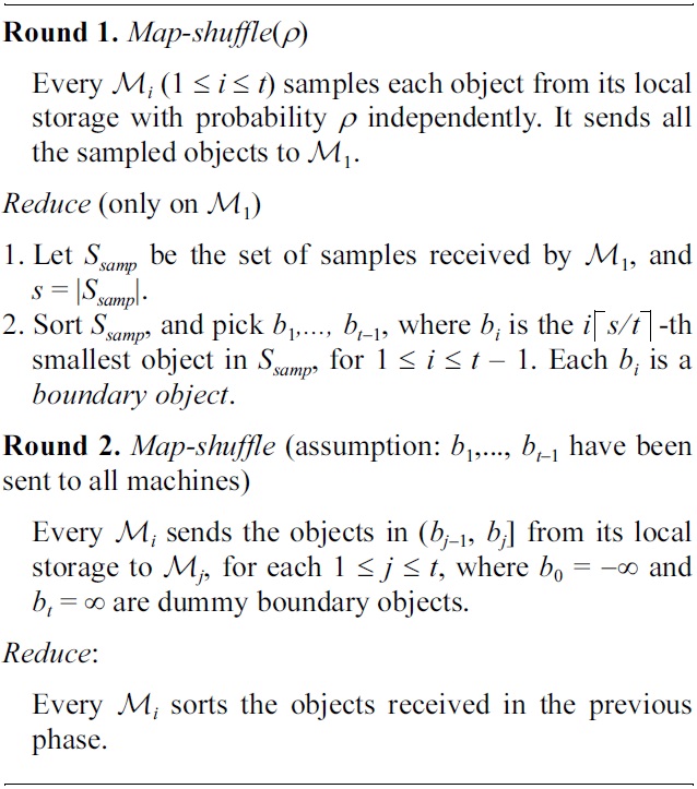
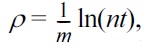
Parameterized by ρ ∈ (0,1], TeraSort [4] runs as follows:

For convenience, the procedure above sometimes asks a machine M to send data to itself. Needless to say, such data “transfer” occurs internally in M, with no network transmission. Also, note the assumption at the map-shuffle phase of Round 2, which we call the broadcast assumption, and will deal with later in Section III-C.

In O’Malley’s study [4], ρ was left as an open parameter. Next, we analyze the setting of this value to make TeraSort a minimal algorithm.

Define S_i = S ？ (b_i？1, b_i], for 1 ≤ i ≤ t. In Round 2, all the objects in S_i are gathered by M_i, which sorts them in the reduce phase. For TeraSort to be minimal, the following must hold:

P1. s = O(m).

P2. |Si|= O(m) for all 1 ≤ i ≤ t.

Specifically, P₁ is necessary because M₁ receives O(s) objects over the network in the map-shuffle phase of Round 1, which has to be O(m) to satisfy bounded net-traffic (see Section I). P₂ is necessary because M_i must receive and store O(|S_i|) words in Round 2, which needs to be O(m) to qualify as bounded net-traffic with a minimum footprint.

We now establish an important fact about TeraSort:

THEOREM 4. When m ≥ t ln(nt), P₁ and P₂ hold simultaneously with a probability of at least

Proof. We will consider t ≥ 9, because otherwise, m = Ω(n), in which case P₁ and P₂ hold trivially. Our proof is based on the Chernoff bound―let X₁,…, X_n be independent Bernoulli variables with Pr[X_i=1] = p_i, for 1 ≤ i ≤ n.

The Chernoff bound states (i) for any 0 < α < 1, Pr[X ≥ (1 + α)μ] ≤ exp(？α²μ/3) while Pr[X ≤ (1 ？ α)μ] ≤ exp(？α²μ/3), and (ii) Pr[X ≥ 6μ] ≤ 2？^6μ―and an interesting bucketing argument.

First, it is easy to see that E[s] = mρt = t ln(nt).

A simple application of the Chernoff bound results in:

Pr[s ≥ 1.6 · t ln(nt)] ≤ exp(？0.12 · t ln(nt)) ≤ 1/n

where the last inequality uses the fact that t ≥ 9. This implies that P₁ can fail with a probability of at most 1/n. Next, we analyze P₂ under the event s < 1.6t ln(nt) = O(m).

Imagine that S has been sorted in ascending order. We divide the sorted list into

sub-lists as evenly as possible, and call each sub-list a bucket. Each bucket has between 8n/t = 8m and 16m objects. We observe that P₂ holds if every bucket covers at least one boundary object. To understand why, note that under this condition, no bucket can fall between two consecutive boundary objects (counting also the dummy ones―if there was one, the bucket would not be able to cover any boundary object). Hence, every S_i, 1 ≤ i ≤ t, can contain objects in at most 2 buckets, i.e., |S_i| ≤ 32m = O(m).

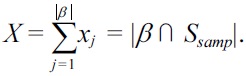
A bucket β definitely includes a boundary object if β covers more than 1.6 ln(nt) > s/t samples (i.e., objects from S_samp), as a boundary object is taken every

consecutive samples. Let |β| ≥ 8m be the number of objects in β. Random variable x_j, 1 ≤ j ≤ |β| is defined to be 1 if the j-th object in β is sampled, and 0 otherwise. Define:

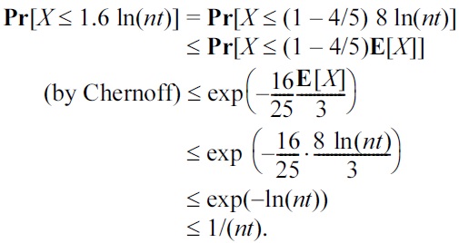
Clearly, E[X] ≥ 8mρ = 8 ln(nt). We have:

We say that β fails if it covers no boundary object. The above derivation shows that β fails with a probability of at most 1/(nt). As there are at most t/8 buckets, the probability that at least one bucket fails is at most 1/(8n). Hence, P₂ can be violated with a probability of at most 1/(8n) under the event s < 1.6t ln(nt), i.e., at most 9/8n overall.

Therefore, P₁ and P₂ hold at the same time with a probability of at least 1 ？ 17/(8n). □

Discussion. For large n, the success probability 1 ？ O(1/n) in Theorem 4 is so high that the failure probability O(1/n) is negligible, i.e., P₁ and P₂ are almost never violated.

The condition about m in Theorem 4 is tight within a logarithmic factor, because m ≥ t is an implicit condition for TeraSort to work, with both the reduce phase of Round 1 and the map-shuffle phase of Round 2 requiring a machine to store t ？ 1 boundary objects.

In reality, typically, m ≫ t, and the memory size of a machine is significantly greater than the number of machines. More specifically, m is on the order of at least 10⁶ (this is using only a few megabytes per machine), while t is on the order of 10⁴ or lower. Therefore, m ≥ t ln(nt) is a (very) reasonable assumption, which explains why TeraSort has excellent efficiency in practice.

Minimality. We now establish the minimality of TeraSort, temporarily ignoring how to fulfill the broadcast assumption. Properties P₁ and P₂ indicate that each machine needs to store only O(m) objects at any time, consistent with a minimum footprint. Regarding the network cost, a machine M in each round sends only objects that were already on M when the algorithm started. Hence, M sends O(m) network data per round. Furthermore, M₁ receives only O(m) objects by P₁. Therefore, bounded-bandwidth is fulfilled. Constant round is obviously satisfied. Finally, the computation time of each machine M_i (1 ≤ i ≤ t) is dominated by the cost of sorting S_i in Round 2, i.e.,

As this is 1/t of the O(n log n) time of a sequential algorithm, optimal computation is also achieved.

Before Round 2 of TeraSort, M₁ needs to broadcast the boundary objects b₁,…, b_t？1 to the other machines. We have to be careful because a naive solution would ask M₁ to send O(t) words to every other machine, and hence, incur O(t²) network traffic overall. This not only requires one more round, but also violates bounded net-traffic if t exceeds

by a non-constant factor.

In O’Malley’s study [4], this issue was circumvented by assuming that all the machines can access a distributed file system. In this scenario, M₁ can simply write the boundary objects to a file on that system, after which each M_i, 2 ≤ i ≤ t, obtains them from the file. In other words, a brute-force file-accessing step is inserted between the two rounds. This is allowed by the current Hadoop implementation (on which TeraSort was based [4]).

Technically, however, the above approach destroys the elegance of TeraSort, because it requires that, besides sending key-value pairs to each other, the machines should also communicate via a distributed file. This implies that the machines are not share-nothing, because they are essentially sharing the file. Furthermore, as far as this paper is concerned, the artifact is inconsistent with the definition of minimal algorithms. As sorting lingers in all the problems to be discussed later, we are motivated to remove the artifact to keep our analytical framework clean.

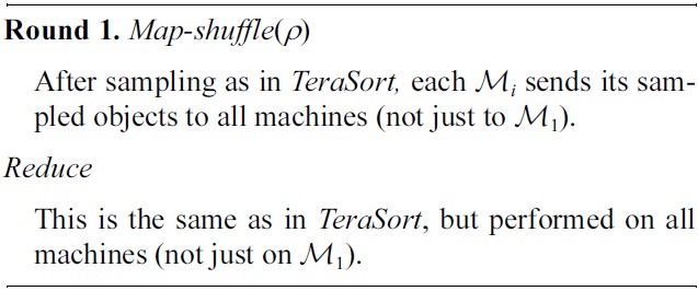
We now provide an elegant remedy, which allows TeraSort to still terminate in 2 rounds, and retain its minimality. The idea is to give all machines a copy of S_samp. Specifically, we modify Round 1 of TeraSort as:

Round 2 still proceeds as before. The correctness follows from the fact that in the reduce phase, every machine picks boundary objects in exactly the same way from an identical S_samp. Therefore, all machines will obtain the same boundary objects, thus eliminating the need for broadcasting. Henceforth, we will call the modified algorithm pure TeraSort.

At first glance, the new map-shuffle phase of Round 1 may seem to require a machine M to send out considerable data, because every sample necessitates O(t) words of network traffic (i.e., O(1) to every other machine). However, as every object is sampled with probability

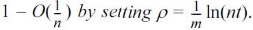
the number of words sent by M is only O(m·t·ρ) = O(t ln(nt)) in expectation. The lemma below gives a much stronger fact:

LEMMA 4. With a probability of at least

every machine sends O(t ln(nt)) words over the network in Round 1 of pure TeraSort.

Proof. Consider an arbitrary machine M. Let random variable X be the number of objects sampled from M. Hence, E[X] = mρ = ln(nt). A straightforward application of the Chernoff bound gives:

Pr[X ≥ 6 ln(nt)] ≤ 2？6 ln(nt) ≤ 1/(nt).

Hence, M sends more than O(t ln(nt)) words in Round 1 with a probability of at most 1/(nt). By union bound, the probability that this is true for all t machines is at least 1 ？ 1/n. □

Combining the above lemma with Theorem 4 and the minimality analysis in Section III-B, we can see that pure TeraSort is a minimal algorithm with a probability of at least 1 ？ O(1/n) when m ≥ t ln(nt).

We close this section by pointing out that the fix of TeraSort is of mainly theoretical concerns. The fix serves the purpose of convincing the reader that the broadcast assumption is not a technical “loose end” in achieving minimality. In practice, TeraSort has nearly the same performance as our pure version, at least on Hadoop, where (as mentioned before) the brute-force approach of TeraSort is well supported.

We have obtained a non-trivial glimpse at the results from research during an appointment with the KAIST. Interested readers are referred previous studies [1,5] for additional details, including full surveys of the literature. Due to space constraints, in this paper, other results have not been described, but can be found online at http://www.cse.cuhk.edu.hk/~taoyf.