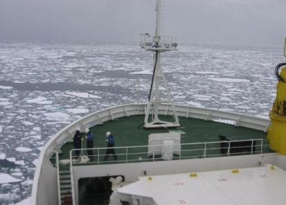
Interest in the Arctic is growing around the world. Global climate change will make the Arctic more attractive for oil and gas activities. The shrinking Arctic ice cover will soon make resources more accessible (Kwok and Cunningham, 2011). Shipping lanes in Arctic waters are opening up, thereby reducing costs and the risks of access. This is advantageous not only for energy companies engaged in oil and gas exploration and production, but also for shipping and ship building/offshore plant companies producing icebreakers and ice cargo vessels. In the near future,a large quantity of the oil and natural gas produced in the Arctic regions of Russia and North America will be supplied to the Northeast Asian region.

According to the increase of northern sea route, the ice going cargo vessels have been moreinvestigated to have efficient performance in ice.Performance in pack ice conditions is important to an ice cargo vessel because normally it follows a sea path covered with pack ice broken by an icebreaker. In the present study, we considered the possibility of using numerical simulation instead of model tests for the analysis of performance in pack ice conditions, especially for time consuming and expensive analysis such as development of the optimum hull form.

A typical ship-ice interaction study is treated as a structural impact analysis with decoupling from hydrodynamic loads for the analysis of resistance performance in pack ice conditions. Combining structural and flow analysis is often prohibitive due to excessive computational cost, and because hydrodynamic loads can be small enough to be considered negligible. Since computational capability has significantly increased and engineering trends can be expected to focus on performance evaluation in ice-laden water, accurate modeling for both flow and structural assessment has become more important. In the past, arctic-class vessels are generally small (LPP of about 100 m), but recent trends are very different. Ship sizes and speeds are increasing. Global warming could drive this trend even faster because Arctic ice is becoming weaker and the year-around shipping area is increasing.

For level ice, Valanto (2001) presented an overview of ship-level ice interaction. They divided the interaction process into several phases: breaking, rotating, sliding, and clearing. Recently, Wang and Derradji (2010) simulated an icebreaker breaking through the level ice using LS-DYNA. They used user-defined ice failure criteria based on the flexural strength. It showed a reasonable agreement with full-scale measurement. Compared to the level ice case, analysis of pack ice conditions is not complex in terms of physics if flexural failure is ignored. Combining structural and flow analysis enables us to assess ships and structures in ice interaction more correctly. Using fluid-structure interaction (FSI) methods, most ice interaction problems can be practically solved; for example, a drill ship in pack ice conditions, lifeboat performance in ice-covered water, and ice management strategies. The LS-DYNA can be used in our analysis has been successfully applied to this class of structural and flow analysis problem (Wang and Derradji, 2010; 2011; Wang and Gagnon, 2012).

To validate the present computational results, experiments were conducted at Pusan National University’s towing tank with synthetic ice under pack ice conditions. There is an analogy between our computations and experimental results with synthetic ice because the fracture failures of ice pieces were not considered in the analysis. Correlation between synthetic and refrigerated ice has also been examined in previous studies (Song et al., 2007; Kim et al., 2009). Experimental results with refrigerated ice from the NRC’s ice tank is also shown for comparison with the experimental results from synthetic ice, and with computational results.

We focused on resistance performance. The total resistance in ice can be divided into four components, as follows (Jones, 1987):

where

Rt = Total resistance in ice.

Rbr = Resistance due to breaking the ice.

Rc = Resistance due to clearing of the ice.

Rc = Resistance due to buoyancy of the ice.

Row = Resistance due to open water.

Level ice tests (an unbroken and solid ice sheet) are normally conducted to measure the total resistance in ice ( R_t ). Presawn ice tests (the ice sheet is cut but the ice pieces are in place) are performed to eliminate breaking resistance; thus, they measure the sum of the clearing, buoyancy, and open water resistance ( R_x + R_b + R_ow ). Since open water resistance ( R_ow ) is known from the resistance tests in open water, the clearing resistance ( R_c ) and buoyancy resistance ( R_b ) are unknown variables in the pre-sawn tests. By conducting the pre-sawn tests at a very low carriage speed such as 0.02 m/s, clearing resistance ( R_c ) due to the ice block rotation, ventilation, and acceleration is negligible. The buoyancy resistance ( R_b ) can be determined with consideration of the effect of the sliding friction only. Therefore, all components can be calculated from Eq. (1). As previously mentioned, in the pack ice condition, the buoyancy, clearance, and open water resistances (except breaking resistance) were considered to be in a pre-sawn ice condition, which is equivalent to 100% concentration in the pack ice condition. The last three components (except breaking resistance) can be expressed as follows:

where R_ps is the resistance in the pre-sawn ice (100% concentration in the pack ice condition).

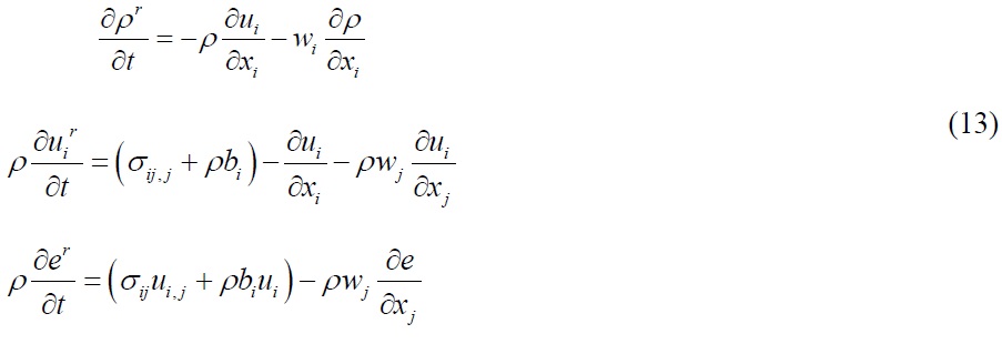
There are several ways to consider a FSI problem numerically. If the structure is treated as a rigid body, then a computational fluid dynamics (CFD) flow solver can integrate the flow velocity field on the wetted surface area and calculate the pressure or drag force (i.e., the ship’s resistance).The disadvantage of using CFD only is having a limited capability of structurestructure interaction, such as ship-ice interaction, as multi-deformable bodies. However the commercial explicit FE solver LSDYNA has the capability to solve the fluid flow using an Eulerian formulation while the structure is considered to be Lagrangian. The arbitrary Lagrangian-Eulerian (ALE) method in LS-DYNA allows for a fully-coupled solution of Lagrangian structures interacting with Eulerian fluids. The principle of the ALE method is that a Lagrangian structure is overlapped on an Eulerian computational domain. At each time step, both the Lagrangian and Eulerian calculations are independently performed and followed by a remapping step (advection step) from the distorted Lagrangian mesh to the Eulerian domain. The last step is interface reconstruction. Since LS-DYNA does not have a full CFD solver (such as a Navier-Stokes solver), hydrodynamic calculations were estimated using a penalty method. The fluid was modeled using dynamic viscosity and equations of state (EOS) with a null material model. The following governing equations were used:

Continuity equation

In fluid mechanics, the continuity equation can be written as

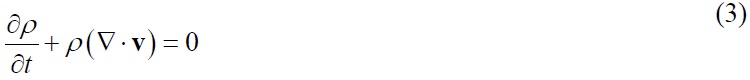
In the material form, Eq. (3) can be written as

Using the Jacobian J, we obtain

Momentum equation

Since the time rate of change of the total momentum of a system is the same as the vector sum of all the external forces, Eq. (5) can be made.

where ρ is the density, t is the surface traction, and b is the body force per unit mass.

Using the Cauchy stress tensor ( σ ), t =σ_ij？n , and the divergence theorem, we have

Energy equation

Using total energy (E), which is the sum of kinetic energy and internal energy, we have

In LS-DYNA, the modified energy equation for the explicit solver Eq. (8) is integrated over time and is used for the equation of state evaluation and a global energy balance:

where V is the relative volume that is the determinant of the Jacobian, p is the hydrostatic pressure, and qis the bulk viscosity. Since the FEM is used to solve the weak form of the momentum equation (using the principle of virtual work), it can be written as Eq. (9):

For time integration, the central-difference method is adopted in LS-DYNA, which is described as

where Δt is the time step size.

In order to formulate an ALE problem, two domains are considered: the material (spatial) domain and the reference domain. The ALE governing equations are derived for the case in which the reference frame moves at an arbitrary velocity. The material velocity is u, the reference frame velocity is v, and their difference, u ？ v, is expressed as w. The basic ALE formulation is given by

where J is the Jacobian, which is the relative differential volume between two domains.

The material time derivatives in the ALE formulation are written as

where b^r means that b is expressed as a function of the reference domain.

Therefore, the ALE equations for the conservation of mass, momentum, and energy are as follows:

In the present computations, AME, a grouping algorithm, and a penalty method were used to simulate the fluid coupling with pack ice based on the preceding governing equations.

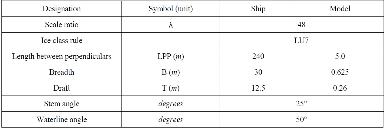
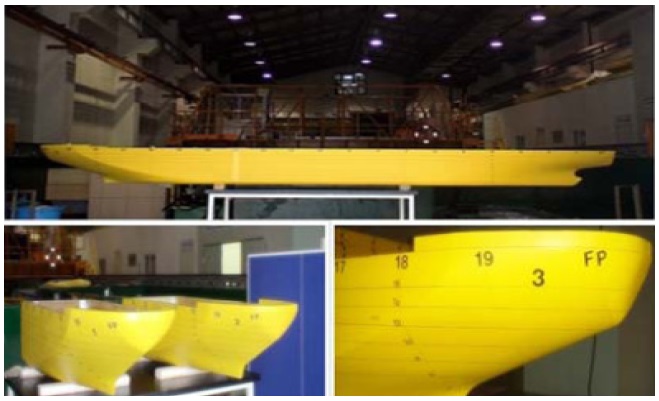
A model ship was designed for this study according to the Russian ice-class rule (LU7). The scale ratio, length, and breadth were set to 48:1, 5 m, and 0.625 m, respectively. The important hull-form parameters for an ice breaking cargo vessel are generally the stem and waterline angles, which are closely related to ice resistance parameters such as clearing and buoyancy forces. In the present experiments, the stem and waterline angles were determined to be 25° and 50°, respectively which are required by the current Russian ice-class rule. Table 1 gives the main parameters of the icebreaking cargo vessel. Fig. 2 shows the model ships.

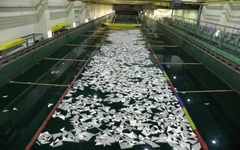
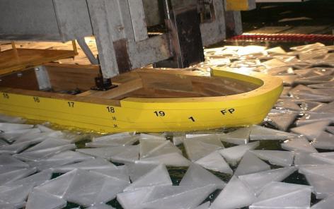
A model test with synthetic ice was conducted in the towing tank of Pusan National University (PNU). The PNU towing tank has dimensions of 100 m in length, 8 m in width, and 3.5 m in depth. For the synthetic ice test, an additional fence was used as shown in Fig. 3, which is the almost same condition of tests in ice tank. The fence is 25 m in length and 3.75 m in width. The fence width was set to six times the model ship width because the fence effect was not to be included.

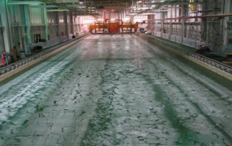
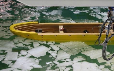
A model test with refrigerated ice was conducted in the ice tank at the Institute for Ocean Technology (NRC) in Canada. The NRC ice tank has dimensions of 91 m in length, 12 m in width, and 3 m in depth, and is shown in Fig. 4. The tank has two carriages and an underwater camera. The ice tank has 24 evaporators using ammonia gas for cooling. The range of the air temperature is from -30 to 15 ℃. The carriage has dimensions of 15 m in length and 14.2 m in width, and weighs 80 tons. The range of the carriage speed is from 0.0002 to 4.0 m/s.

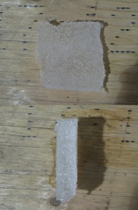
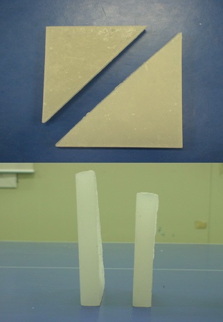
Synthetic ice was made from fragments of semi-refined paraffin wax. A lump of paraffin wax was melted and poured into triangular frames for the desired shape. The synthetic ice had an average thickness of 20 mm, an approximate relative density of 0.87, and a friction coefficient of 0.03 (the frictional coefficient of refrigerated ice is 0.01). Two sizes of triangular-shaped wax were used: 160 and 110.5 cm². The triangular shape tends to regulate concentration in the pack ice condition. Since breaking or cracking of the ice was not taken into account in our tests, the strength of the model ice may not be significant, as previously mentioned. The profile of the synthetic ice is shown in Fig. 5 (Lee et al., 2009).

The refrigerated ice used in this study was based on the EG/AD/S model, which is specially designed to provide the scaled flexural strength of columnar sea ice (Timco, 1986). It is a diluted aqueous solution of ethylene glycol (EG), aliphatic detergent (AD), and Sugar (S). The profile of the refrigerated ice, which had a thickness of 20 mm, is shown in Fig. 6. Table 2 shows a comparison between refrigerated ice and synthetic ice.

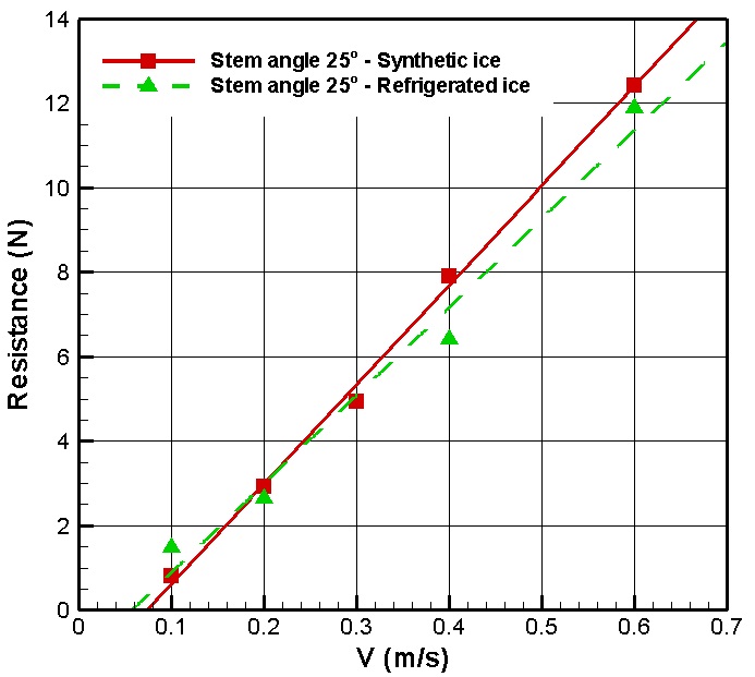
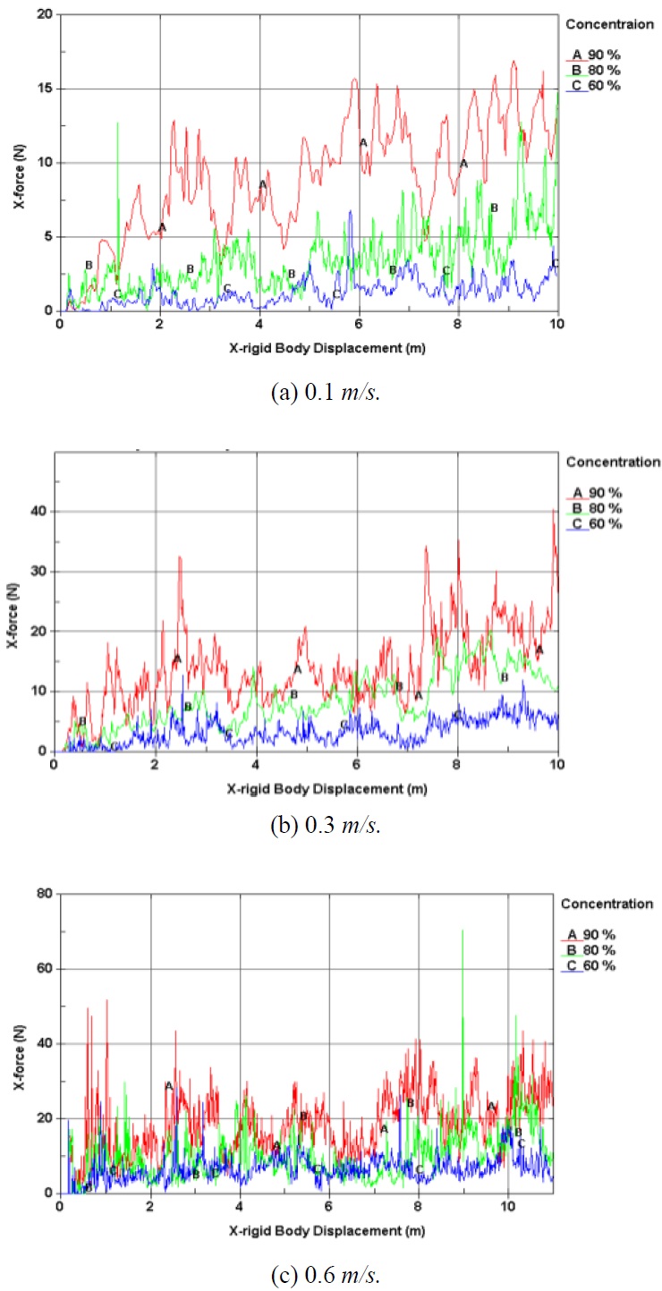
Resistance tests under three pack ice conditions were performed at both the NRC ice tank using refrigerated ice and the PNU towing tank, using synthetic ice at four model speeds (0.1, 0.3, 0.4, and 0.6 m/s). Photos of the towing tank and ice tank are shown in Figs. 7, 8, and 9.

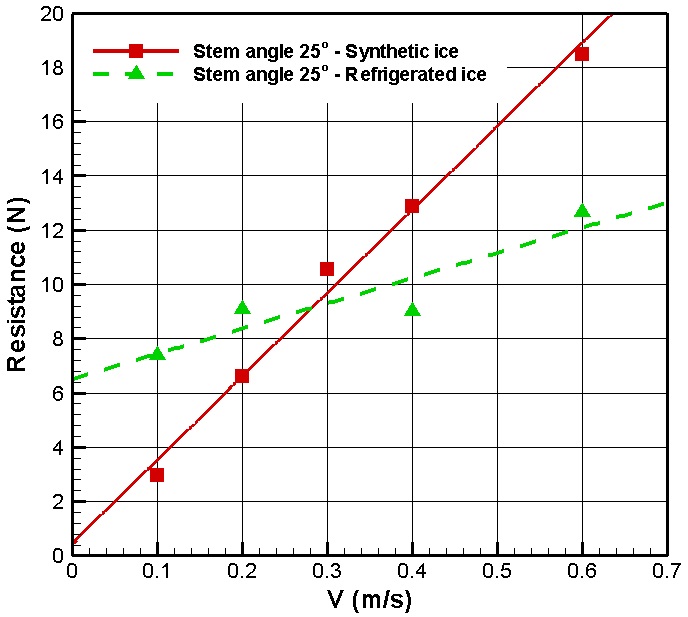
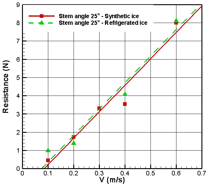
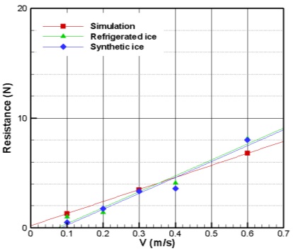
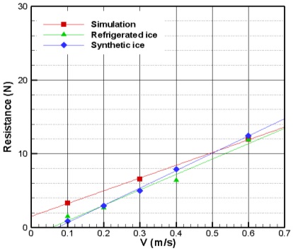
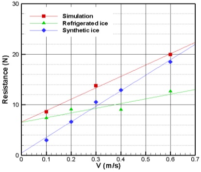
The results from the resistance test with three different pack ice concentrations (90%, 80%, and 60%) are shown in Figs. 10-12, respectively. These results have all similar tendencies from the all concentration of 90%, 80% and 60%. The synthetic ice results were compared to the refrigerated ice results to find a correlation. For concentrations of 80% and 60%, the results of the PNU resistance test are in good agreement with the results from the NRC resistance test, both qualitatively and quantitatively. There is some discrepancy in the case of 90% concentration between the refrigerated ice and the others due to the uncertainty of the interaction between the hull and the randomly-distributed ice pieces. According to these comparisons, there might be possibility that refrigerated ice is replaced by synthetic ice in the pack ice condition.

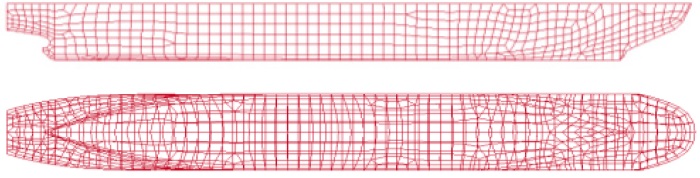
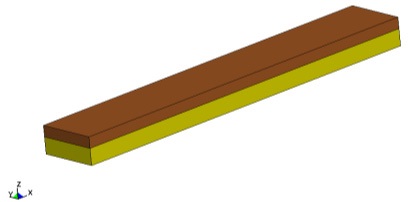
Numerical simulations of a collision between pack ice and a model ship were conducted using LS-DYNA software. The results compared favorably with actual data acquired during tests in the NRC ice tank using real ice and the PNU towing tank using synthetic ice (Gagnon, 2007). The modeled volume including the ice, water, and model ship was meshed using ANSYS^® software and contained approximately 100,000 elements. Fig. 13 shows a panel model of an icebreaking cargo ship, and Fig. 14 shows the modeled region of the water and air including the model ship and ice pieces. The dimensions of the air/water region were 20 m long × 3 m wide ×0.9 m deep. The top 0.6 m was air.

For each case, the nominal element size was about 0.08 m. The ice floe shapes were a right triangle with dimensions of 0.16 m × 0.13 m and 0.20 m × 0.16. In order to maintain the given concentration, rigid frames on both sides and at the far end were used. We note that these rigid frames did not interact with the water and air, but did interact with ice blocks. LS-DYNA contains many material types that can be applied to objects within the simulation. In our simulation, the model ship was treated as a rigid body. Similar results would have been obtained if the model ship’s shell elements were given elastic properties similar to steel. However, the simulation was run with the model ship as a rigid body in consideration of computing time and the small size of the pack ice. For the ice pieces, likewise, we assumed that the pack ice conditions did not have much breaking or crushing behavior, but did have a clearing and pushing away effect from the ship at the water’s surface. For this reason, we modeled the ice as a rigid body. Fig. 14 shows our modeling of the ice pieces. At the end of the wave tank, ambient elements with a pressure inflow condition (acting as a non-reflecting boundary) were inserted to avoid any reflecting wave that could disturb the newly-generated wave from the wave ship. Figs. 15 and 16 show the modeling of ice pieces and the tank condition, respectively. 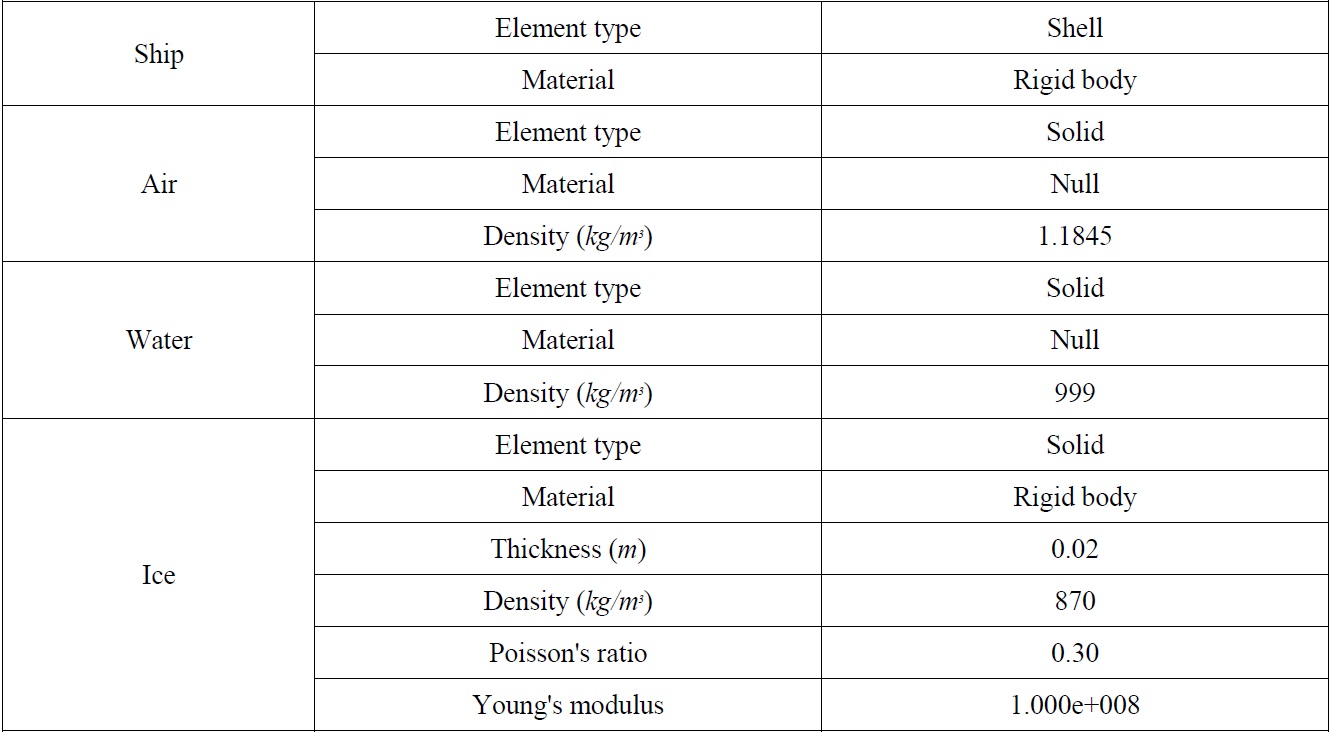Table 3 lists simulation parameters and values for the simulations.

To ensure that the water and the objects behaved correctly during the simulations, gravity was applied to the mesh elements. This was done by applying an acceleration equivalent to the acceleration of gravity to all elements in the meshed model. This resulted in the proper hydrostatic pressure gradient developing in the water early in the simulation, created the proper buoyant forces on floating objects, and enabled the formation of waves on the free surface of the water. In LS-DYNA, two objects and materials can overlap each other within a volume of the mesh, which can introduce errors in the simulation. Hence, it is necessary to ensure that when the model ship and the ice pieces are added to the LS-DYNA k-file, the water is removed from the volume to be occupied by each object. This is easily done for shell objects (such as the model ship) within LS-DYNA by using the command “initial-volume fraction”. Fig. 17 shows the volumes of the air part and the water part. (LS-DYNA theoretical manual, 2006; Hallquist, 2007)

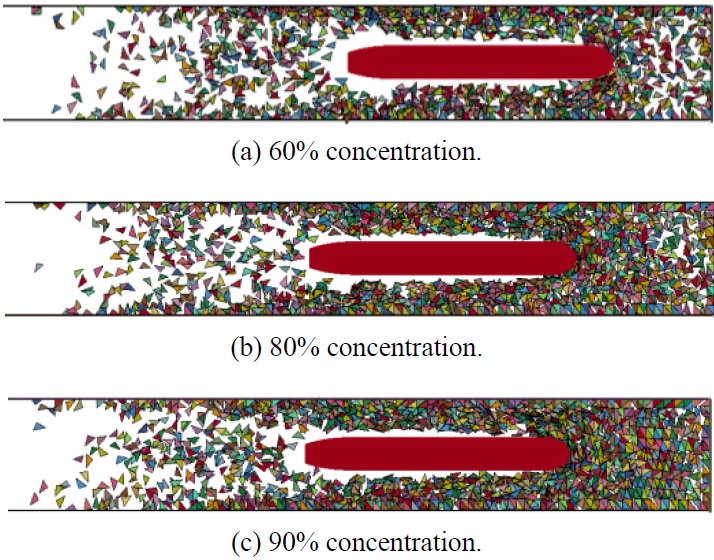
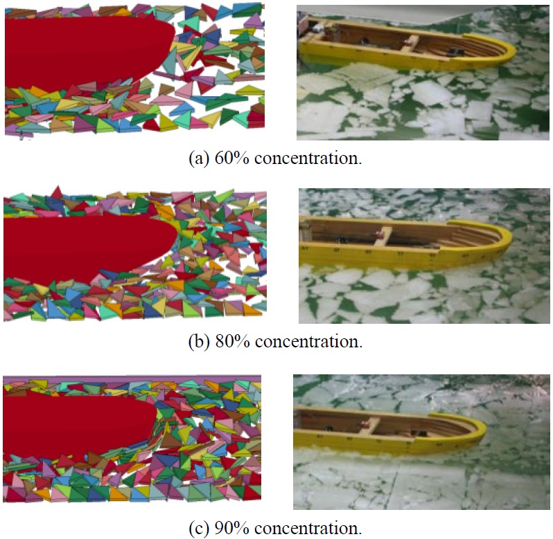
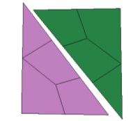
Fig. 18 shows concentrations of the pack ice condition (60%, 80%, and 90%) wherein the concentrations are defined by the ratio of the area covered by rectangular pack ice and the whole water surface. The pack ice was randomly distributed, as in the experimental condition.

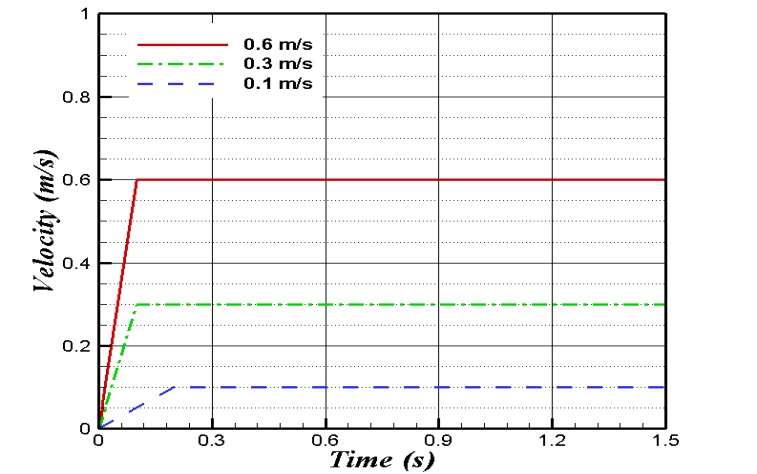
The maximum speed of the model ship was set to 0.6 m/s, which is equivalent to 8.08 knots in a full-scale ship. In order to obtain the performance trend according to the variation of speed, 0.1and 0.3 m/s were chosen combined with the 60%, 80%, and 90% concentration conditions. Fig. 19 shows the profile of the speed variation used in the computation, which prevented an unrealistically large acceleration upon starting.

The contact forces evolved as the motions required, and they were determined solely based on reactions. These forces were calculated by solving the equations of motion of the unbreakable ice pieces. Both static and dynamic friction were included in the contact formulations. At every time step, we used the previous positions of the ice pieces and the current position of the ship to detect contacts among the ice pieces, and between the ice pieces and the ship's hull. We also used the previous positions of the ice pieces to calculate the buoyancy forces acting on these pieces. The gravitational forces were calculated and applied to each piece at its center of mass. The model ship calculated the clearing force component by considering the force imposed by the motion of an ensemble of ice pieces rotating and sliding along the submerged surface of the hull. The clearing force component includes viscous drag and inherent buoyancy for the rotating ice floes, forces caused by wave pressure and ventilation of the rotating ice floes, and inertial forces due to ice acceleration (Raed and Sveinung, 2011).

Fig. 20 shows the results of the simulation at concentrations of 60%, 80%, and 90%. Interaction between the hull and ice occurred frequently according to the increase in concentration, as shown in Fig. 21. For the simulation of 80% and 90% concentrations, ice pieces were stuck on the shoulder of the ship, which caused a large load lasting approximately 2 to 3s.

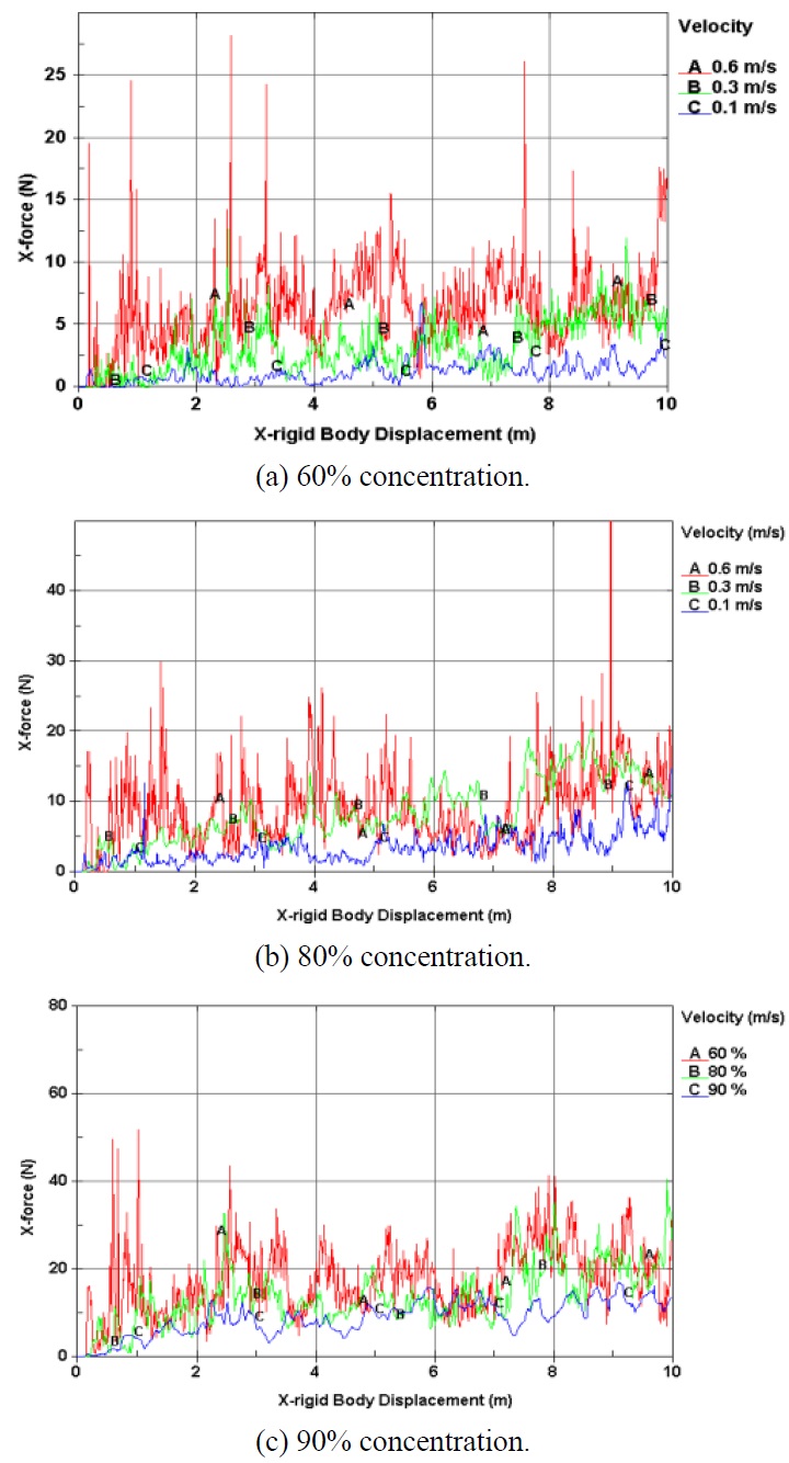
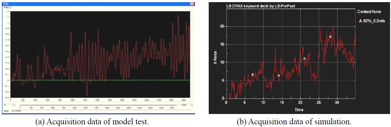
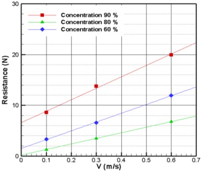
Figs. 22 and 23 show the computed surge forces according to the advanced distance at each concentration and ship speed. The forces increased slightly according to the ship’s advance due to accumulated ice, which is similar to the experimental results shown in Fig. 24. The averaged surge force increased according to the increase in concentration and ship speed, as expected. To clearly see the trend of the average amount of resistance (the surge force) at each speed, the resistance was calculated during the previously shown data by cutting the parts of from 2 m of starting point and end point. Fig. 23 shows the calculated average resistances at each ship speed (0.1, 0.3, and 0.6 m/s) according to the variation of concentration.

The computed results are compared to the experimental results from synthetic ice and refrigerated ice in Figs. 25-28. There is good correspondence among the three cases with respect to uncertainty in the interaction of the hull and randomly distributed ice. There is some difference only in the refrigerated ice case (90% concentration) compared to the other data. The trend and value of the refrigerated ice case at 90% concentration seems somewhat different than other data.

We introduced a numerical method to simulate ship resistance performance in pack ice conditions. The effect of the ship’s motion was considered for the calculation of ice forces acting on ship, and the rigid body equations of surge were solved by numerical integration. Ship-ice interaction loads for pack ice conditions were numerically calculated based on the fluid structure interaction (FSI) method using the LS-DYNA commercial FE package .Our numerical analysis was validated by comparison with model ship performance data from the PNU towing tank and NRC ice tank. The simulated results are in good agreement with experimental results overall, both qualitatively and quantitatively. This is probably due to the fact that there was no failure in the pack ice pieces; otherwise, the fracture strength and modeling of the ice pieces might be important in the analysis. Our comparison shows the possibility of applying the proposed numerical computation to an analysis of the pack ice condition. The proposed approach might be especially effective as a replacement for time-consuming hull form optimization instead of experiments in an expensive ice tank. As the next research step, a proper ice model (using a deformable body) with more realistic ice geometry and an improved boundary set-up will be considered in order to increase realism and accuracy. For additional validation of the present study, more comparison data will be accumulated, and a comparative study with full-scale data is expected to be performed in the near future.