Recently, a large class of financial engineering problems dealing with index tracking and portfolio optimization have been considered as an important application domain for several types of engineering and applied mathematics principles [1-8]. Because this class can be conveniently viewed and formulated as an optimal decision-making problem in a highly uncertain and stochastic environment, particularly pertinent to this problem are approaches based on stochastic optimal control methods. The stock index tracking problem is concerned with constructing a stock portfolio that mimics or closely tracks the returns of a stock index such as the S&P 500. Stock index tracking is of practical importance since it is one of the important methods used in a passive approach to equity portfolio management and to index fund management. To minimize tracking error against the target index, usually full replication, in which the stocks are held according to their own weights in the index, or quasi-full replication is adopted by the fund managers. An exchange traded fund (ETF) is a good example of such portfolio management since it is constructed according to its own portfolio deposit file (PDF). Such a full replication or quasi-full replication can be very costly owing to transaction and fund administration costs. The constrained index tracking considered in this paper is concerned with tracking a stock index by investing in only a subset of the stocks in the target index under some constraints. Because it uses only a subset of the stocks and is expected to dramatically reduce the management costs involved in index tracking and simplify portfolio rebalancing more effectively, this problem is particularly important to portfolio managers [7]. Successfully constrained index tracking is also expected to increase the liquidity of an ETF since we may be able to construct the same ETF without investing in the same quantity of stocks in its PDF. To achieve good tracking performance with a subset of stocks in the index, several methods (e.g., control theory [1,4], use of genetic algorithms [3], and evolutionary methods [2]) have been studied by researchers.
In this paper, we consider the use of approximate dynamic programming (ADP) for solving the constrained index tracking problem. Recently, the use of ADP methods has become popular in the area of stochastic control [9-12]. As is well known, solutions to optimally controlled stochastic systems can be well explained by using dynamic programming (DP) [9,10]. However, stochastic control problems cannot be solved by DP exactly except in very simple cases, and to obtain good suboptimal policies, many studies rely on ADP methods. ADP methods have been successfully applied to many real-world problems [13], including some financial engineering problems such as portfolio optimization [5,11,12]. The main objective of this paper is to extend the use of ADP to the field of index tracking. More specifically, we (slightly) modify a mathematical formulation of the constrained index tracking problem in [1,4] and establish an ADP-based procedure for solving the resultant stochastic state-space control formulation. Simulation results show that this procedure works well when applied to real financial market data.
The remainder of this paper is organized as follows: In Section 2, preliminaries are provided regarding constrained index tracking and ADP. In Section 3, we describe our main results from an ADP-based control procedure for the constrained index tracking problem. In Section 4, the effectiveness of the ADPbased procedure is illustrated by using real financial market data. Finally, in Section 5, concluding remarks are presented.
In this paper, we examine constrained index tracking based on ADP. In the following, we describe some fundamentals regarding constrained index tracking and ADP.
2.1 Constrained Index Tracking Problem
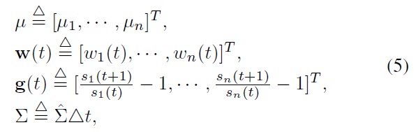
In this section, we describe a constrained index tracking problem [1,4], in which an index of stocks is tracked with a subset of these stocks under certain constraints, as a stochastic control problem. We consider the index

where

is the drift of the
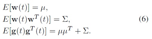
is a vector Brownian motion satisfying

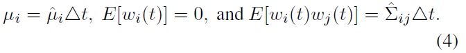
By performing discretization using the Euler method with time step Δ

where
Note that with
we have
Further, note that with
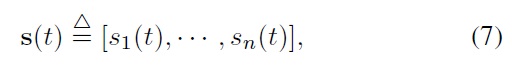
the index value defined by a weighted average can be expressed as
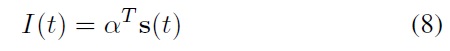
for some
Without loss of generality, in this paper we assume
i.e., the index

Extending the results of this paper to a general
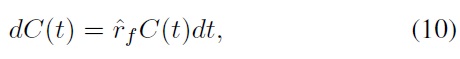
where

is the risk-free rate [14]. When the time step is Δ
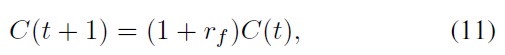
where
[14]. We assume that the money amounts of the first

Note that it is the total value of this portfolio vector that should track the index value over time. More precisely, our goal is to let the wealth of our portfolio,

approach sufficiently close to the index value

where
2.2 Approximate Dynamic Programming
Dynamic programming (DP) is a branch of control theory concerned with finding the optimal control policy that can minimize costs in interactions with an environment. DP is one of the most important theoretical tools in the study of stochastic control. A variety of topics on DP and stochastic control have been well addressed in [9-12]. In the following, some fundamental concepts on stochastic control and DP are briefly summarized. For more details, see, e.g., [11]. A large class of stochastic control problems deal with dynamics described by the following state equation:

where x(

that can optimize a performance index function. A widely used choice for the performance index function of infinite-horizon stochastic optimal control problems is the expected sum of discounted stage costs, i.e.,
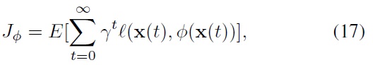
where
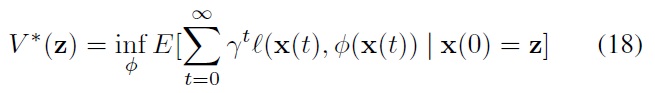
According to optimal control theory [9,10], the state value function

and an optimal control policy

In its operator form, the Bellman equation can be written as

where

for any
By applying this strategy to Eq. (20), one can find a suboptimal control policy

In this paper, we apply this ADP strategy to the constrained index tracking problem.
3. ADP-Based Constrained Index Tracking
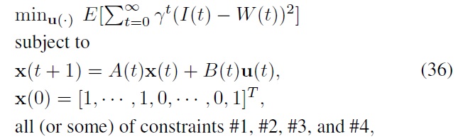
In this section, we describe constrained index tracking in the framework of a stochastic state-space control problem, and we present an ADP-based procedure to find a suboptimal solution to the problem. To express the constrained index tracking problem in a state-space optimal control format, we need to define the control input and state vector together with the performance index that is used as an optimization criterion. The control input we consider for the constrained index tracking problem is a vector of trades,
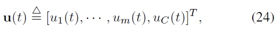
executed for the portfolio
y(t)?[y1(t),· · · , ym(t); yC(t)]T
at the beginning of each time step

With these state and input definitions, the state transition of Eq. (14) can be described by the following state equation:

where
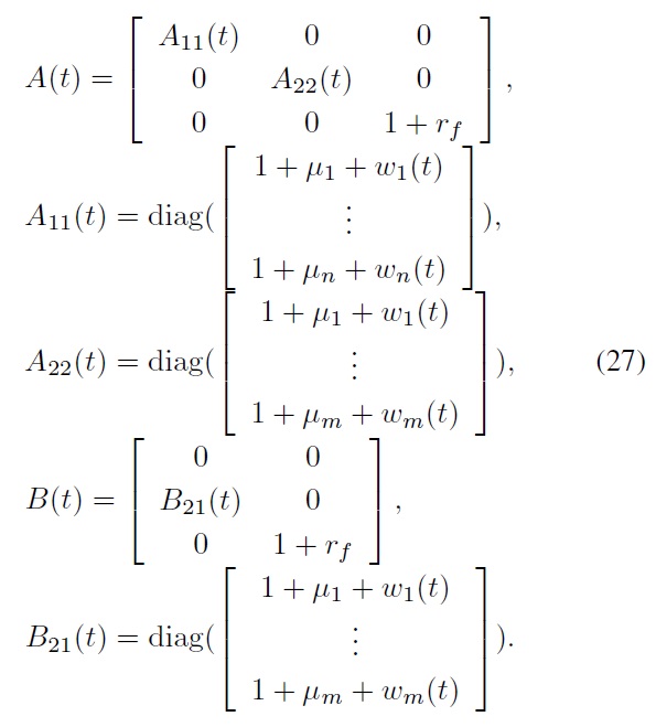
As in [1], we assume that our stock prices are all normalized in the sense that initially they start from

A commonly used distance function for index tracking is the squared tracking error [1], i.e.,

Note that in this performance index function, both

which means that the tracking portfolio starts from the all-cash initial condition with a unit magnitude. With the above statespace description, the problem of optimally tracking the index,
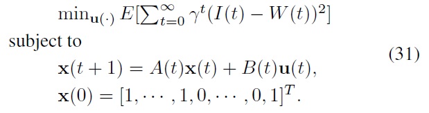
In solving this index tracking problem, the tracking portfolio y(

which means that the total money obtained from selling should be equal to the total money required for buying. Next, we impose a nonnegativity (i.e., long-only) condition for our tracking portfolio, i.e.,

for ∀

where the
where

are used for approximating state value functions, and letting parameters of the

satisfy a series of Bellman inequalities

with
guarantees that

is a lower bound of the optimal state value function
In this paper, we obtain an ADP-based solution procedure for the constrained index tracking problem of Eq. (36) utilizing the iterated-Bellman-inequality strategy [11,12]. To compute the stage cost, we note that since the initial stock prices and the initial cash amount are both normalized (i.e.,
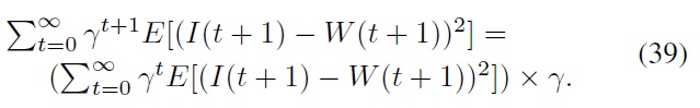
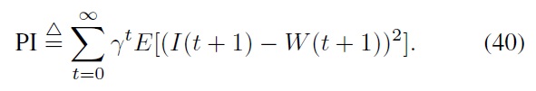
For simplicity and convenience, we use the first term on the right-hand side of Eq. (39) as our new performance index function, i.e.,
Now we consider the tracking error at time

Then the tracking error
Based on this equality, one can obtain an expression for the stage cost, i.e., the expectation of the squared tracking error at time step (
as follows:
where
Note that here the
Now we let the
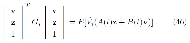
Here, the expectation in the right-hand side is equal to
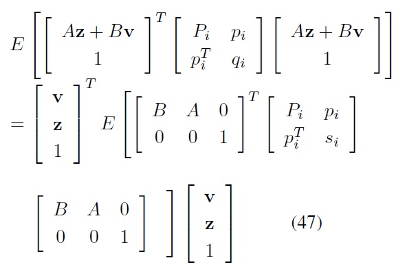
Then, by evaluating the right-hand side of Eq. (47), we obtain
where
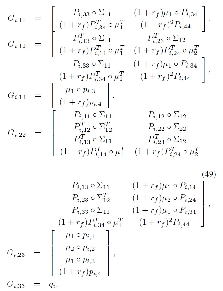
In Eq. (49), the
and ? denotes the elementwise product.
Note that the constraints considered in this paper are all linear. Hence, the left-hand sides of our constraints can be expressed as
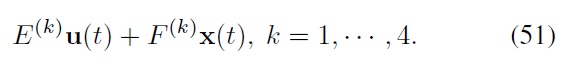
More specifically, the first constraint can be written as
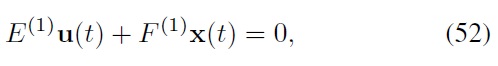
where
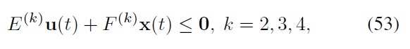
where
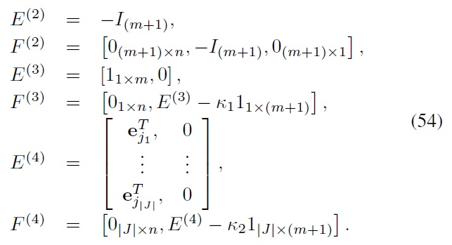
Note that, in Eq. (54), the allocation constraint set
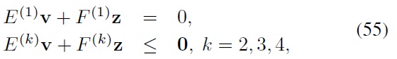
we must have
where
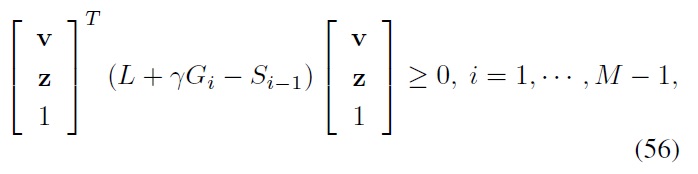
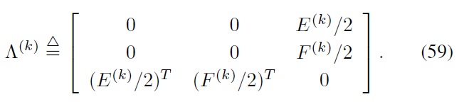
Finally, note that one can obtain the following sufficient condition for the constrained Bellman inequality requirement in Eqs. (55) and (56) using the
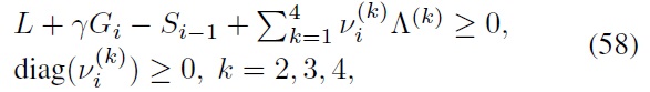
where the

are
By combining all the above steps together, the process of finding a suboptimal ADP solution to the constrained index tracking problem can be summarized as follows:
[Procedure]
1. Choose the discount rate γ and the allocation upper bounds κ1 and κ2.
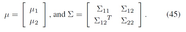
2. Estimate μ, Σ, and rf .
1. Initialize the decision-making time
2. Compute the stage cost matrix
3. Observed the current state x(
4. Define LMI variables:
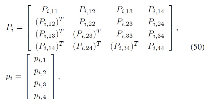
(a) Define the basic LMI variables, Pi, pi, and qi of Eq. (37).
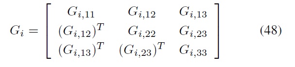
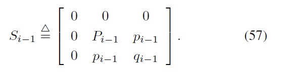
(b) Define the derived LMI variables, Gi of Eq. (48) and Si of Eq. (57).
(c) Define the S-procedure multipliers,
of Eq. (58).
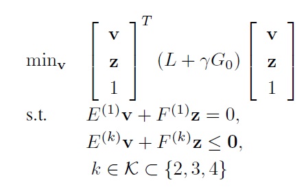
5. Find an approximate state value,

by solving the following LMI optimization problem:
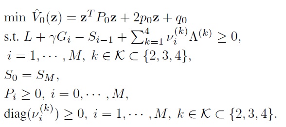
6. Obtain the ADP control input, u(
and trade accordingly.
7. Proceed to the next time step, i.e.,
8. (optional) If necessary, update
9. Go to step 2.
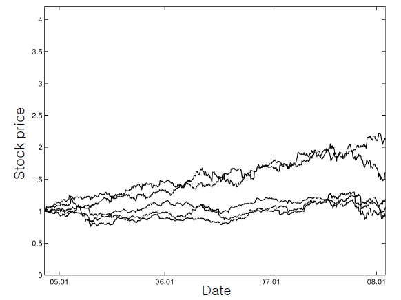
In this section, we illustrate the presented ADP-based procedure with an example of [1], which dealt with daily prices of five major stocks from November 11, 2004, to February 1, 2008. The index
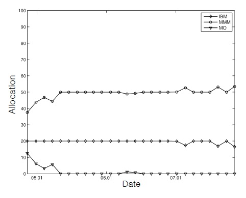
As the subset comprising the tracking portfolio, the first three stocks,
as in [1]. Between each 30-day update, the number of shares in the tracking portfolio remained the same. The ADP discount factor was chosen as
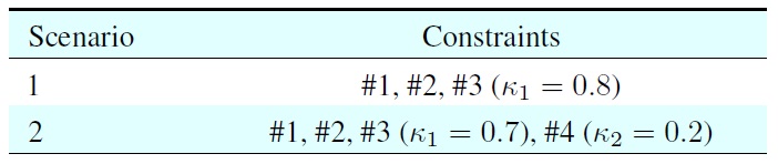
[Table 1.] Simulation scenarios

Simulation scenarios
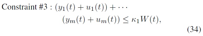
As described in Section 3, the performance index function was computed based on the mean-square distance between the index and the portfolio wealth. Finally, the allocation upper bound was considered for the first stock (i.e.,
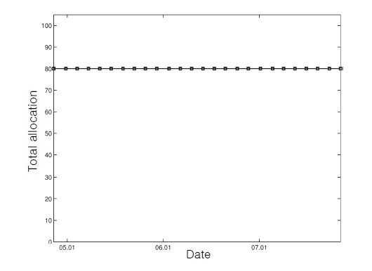
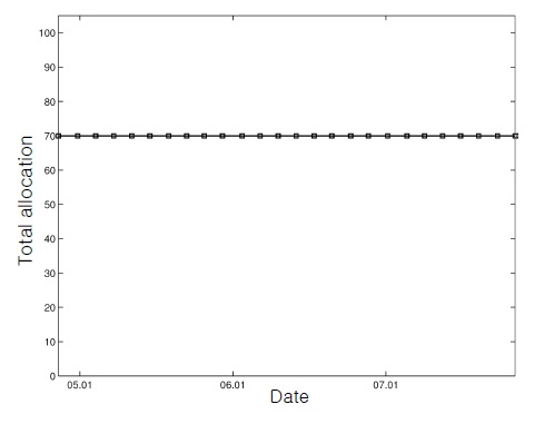
We considered two scenarios with different constraints (Table 1). As shown in Table 1, trading has more severe constraints as the scenario number increases. In the first scenario, we traded with fundamental requirements (i.e., self-financing and a nonnegative portfolio) and the total allocation bound constraint (i.e., Constraint #3). For the upper bound constant for constraint #3, we used
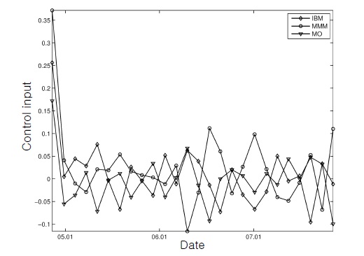
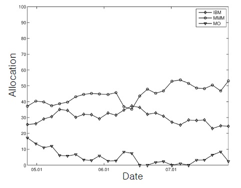
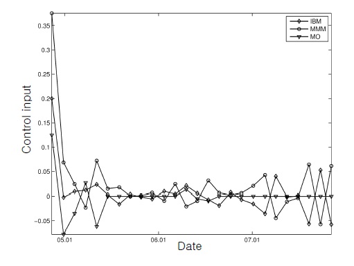
This figure, together with Figure 2, shows that the control inputs changed the initial cash-only portfolio rapidly into the stock-dominating positions for successful tracking.
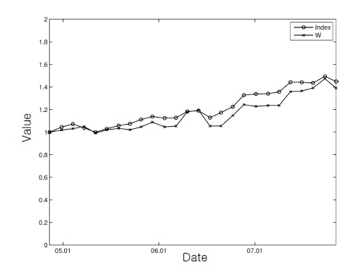
In the second scenario, more difficult constraints were imposed. More specifically, the
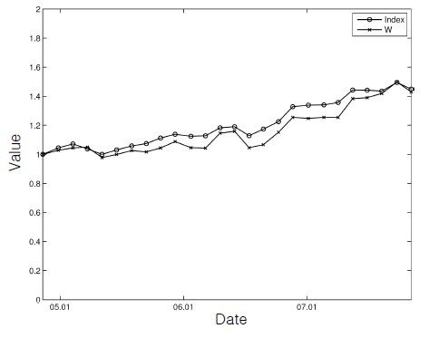
These figures show that, although the tracking performance was a little degraded owing to the additional burden, the wealth of the ADP-based portfolio followed the trend of the index most of the time reasonably well with all the constraints being respected.
The constrained index tracking problem, in which the task of trading a set of stocks is performed so as to closely follow an index value under some constraints, can be viewed and formulated as an optimal decision-making problem in a highly uncertain and stochastic environment, and approaches based on stochastic optimal control methods are particularly pertinent. Since stochastic optimal control problems cannot be solved exactly except in very simple cases, in practice approximations are required to obtain good suboptimal policies. In this paper, we studied approximate dynamic programming applications for the constrained index tracking problem and presented an ADP-based index tracking procedure. Illustrative simulation results showed that the ADP-based tracking policy successfully produced an index-tracking portfolio under various constraints. Further work to be done includes more extensive comparative studies, which should reveal the strengths and weaknesses of the ADP-based index tracking, and applications to other types of related financial engineering problems.
No potential conflict of interest relevant to this article was reported.