Recent innovations in wireless technology have contributed to the rapid growth of wireless communication such as cellular and multi-hop wireless networks. Multihop wireless networks are considered to play an especially important role in communications due to their mobility and flexibility. Examples are wireless mesh networks being considered for the replacement of the backbone network [1], vehicular ad-hoc networks creating the connectivity between moving cars [2], wireless sensor networks monitoring and tracking the environment or the target remotely [3], and mobile ad-hoc networks that selforganize without infrastructure aid [4]. One considerably attractive network is the mobile ad-hoc network (MANET), which creates dynamical arbitrary topologies due to node mobility. Since multi-hop wireless networks create conectivity without a pre-existing infrastructure, they have been considered in the deployment of many applications involved in difficult or dangerous tasks where the network infrastructure may not be available. For example, network infrastructure may not be available on the military battlefield, during disasters, or in a rescue environment. A MANET can also be used to provide extended connectivity for the coverage increments in a cellular network or wireless health monitoring system. Such a network requires cooperative nodes willing to act as a router because the wireless link is determined by the receiving signal strength, which is affected by node mobility and interference.

The topology changes with dynamical link changes and adaptive route establishment is required in a multi-hop wireless network. Therefore, connectivity is essential.

In a multi-hop wireless network, connectivity should be maintained to maintain communication because of dynamical topology changes. The network is known to be connected if all pairs of nodes have at least one path, while the network is not connected or partitioned if at least one pair of nodes does not have a path. Note that pre-determined network design is not possible where a wireless link is susceptible to node mobility and interference. Therefore, maintaining connectivity in a multi-hop wireless network is challenging because of its unstructured topology, link and node failure, unreliable wireless channel properties, and limited battery life [1-4].

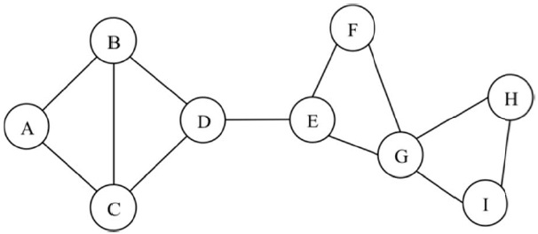
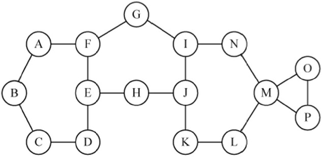
Here we provide an approach to improving the network connectivity to increase the reliability of a given multi-hop wireless network. For a given connected network, we identify the weak or critical points of the network and strengthen those critical points to improve the network survivability. In a multi-hop wireless network, a critical point can be a link, node, or combination of them that partitions the network topology into two or more due to its failure. A link whose failure partitions the network is defined as a critical link, and it is also called a bridge link in a network graph. A node that partitions the network when it fails is defined here as a critical node and is also known as an articulation node. In Fig. 1, for example, link D-E and node G are critical points. The link D-E is a critical link because the network partitions into two network clusters (i.e., A-B-C-D and E-F-G-H-I). Similarly, when node G fails, the network is broken into two clusters, A-B-C-D-E-F and H-I.

In a traditional wired network, a backup route is utilized for the network survivability where the backup route can be link or node disjoint. The backup route allows the network to remain connected in any circumstance of link or node failure. For the network that is still connected from simultaneous failure of (k-1) number of nodes, at least k node disjoint routes for each pair of nodes are required. The network is k-connected if and only if each pair off nodes has at least k disjoint routes. In a multi-hop wireless network, a k-connected network topology is also recommended to prevent a network partition from node or link failure. In order to achieve k-connectivity, many studies have investigated how k-connectivity can be inferred probabilistically or estimated in multi-hop wireless networks [4,5,7-9]. Most of these studies have focused on topological control by transmission power based on node density to accomplish k-node connectivity for a homogeneous wireless network. Bettstetter [7] looked into this problem by identifying the behavior off a minimum node degree for the minimum transmission range. He identified the minimum node degree to maintain k-connectivity of the network topology that uniformly distributed homo-geneous nodes within a limited deployment area. the work was extended in [8]. Ling and Tian [8] develop a probabilistic upper and lower boundary of a k-connected network for the transmission range and node density. Their study is based on the relationship between the node degree and probability of being k-connected [7]. Zhang and Hou [9] propose a transmission power control technique to maintain the k-connectivity via a mathematical approach. They reduce the total transmission power to maintain k-connectivity with ann assumption based on the relationship of minimum node degree and k-connectivity in [7]. Recent studies [7-9] have looked at k-connectivity using the node degree theoretically; however, it can be ensured in very high node density, which would generate a large interference and lower the throughput. Thus, those results are not adequate for sparse to medium-sized multi-hop wireless networks [10].

In a k-connected network, each node has at least k neighbor nodes (i.e., the minimum node degree ≥ k). However, a network in which the minimum node degree is k (i.e., k neighbor nodes) does not guarantee a k-connected network. Although the minimum node degree creates more connectivity, critical connectivity points that partition the network graph may still exist. Therefore, maintaining a minimum node degree of k is a necessary butt not sufficient condition for a k-connected network. Recently, a few papers have begun to look into this problem by defining and identifying the critical points of multi-hop wireless networks. The depth first search algorithm (DFS) is proposed in [11], and it only finds the critical links where the critical node is out of scope in that paper. For a better algorithm, Milic and Malek [12] propose the distributed breadth first search algorithm (dBFS) to detect the critical node and link utilizing distributed computation. In [13], critical node and link detection heuristics are proposed and they utilize local topology and location information. Their proposed algorithm is to find the critical points using a sub-network graph created by eliminating incident links. If the sub-network is not connected, then it is a critical point. As noted in [13], locally detected critical points may not be global critical points due to the existence of alternate routes outside the local topology information. In [14], we proposed a critical point identification algorithm and topology control resilient schemes. The critical point identification algorithm is based on results from algebraic graph theory, namely the algebraic connectivity of the network topology graph. The proposed algorithm requires global connectivity information, which can result in significant communication overhead.

In this paper, we propose a novel algorithm for identification of critical points in a network. The approach is based on examining the connectivity between neighbor nodes without global connectivity information. In many cases, obtaining network topology may not be easy while obtaining limited sub-network information may be relatively easy. Therefore, we also introduce how each node makes its decision on critical points based on H-hop neighbor node information. These H-hop local critical points can be used to predict multiple critical points and global critical points. Using the critical nodes identified by our algorithm, we propose two techniques to improve the survivability of the network by removing the H-hop local critical points. The basic idea is adjusting the transmission power of individual neighbor nodes around a critical point in order to create additional backup links between the nodes. The rest of the paper is organized as follows. In Section II, the proposed critical point detection algorithm is presented, along with implementations for H-hop local critical points and multiple critical points. We also propose two resilient techniques to strengthen the network around critical points. Simulation results illustrating the effectiveness and tradeoffs of the resilience schemes are given in Section III. Lastly, we present our conclusions in Section IV.

In this section, we provide the notation used in the paper. Then, we present the proposed heuristic critical point identification algorithm.

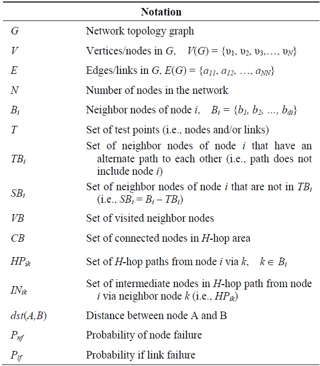
We consider an arbitrary multi-hop wireless network of N nodes. At any point in time, the topology can be represented by a graph G consisting of a set of vertices/nodes V, and edges/links E. For simplicity, a homogeneous wireless network is assumed, where nodes have identical properties and inhabit a uniform environment (e.g., identical battery life, transmission power, antennas, radio propagation ranges, etc.). Table 1 lists our notation.

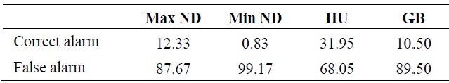
In wired networks, the concept of identifying critical network nodes has recently been investigated from an infrastructure protection standpoint [15,16]. This literature focuses on which nodes will have the most impact on the network (in terms of connectivity or traffic loss) and a variety of heuristics have been proposed to identify the critical nodes, such as maximum degree nodes and maximum traffic nodes. In this section, some simple heuristics in identifying critical nodes are examined for their effectiveness; specifically, we consider the maximum node degree (Max ND), minimum node degree (Min ND), most heavily utilized (HU) nodes (i.e., nodes on the greatest number of shortest primary path routes), and nodes having the greatest backup path (GB) routes passing through them. The backup path routes are node disjoint with the shortest path primary route for each pair of nodes.

In evaluating the heuristics in the literature, we tested 100 connected random topologies that contained at least one critical node. The topologies were created by randomly placing 50 nodes each with 250 m of communication range in an area of 1,000 m × 1,000 m. Table 2 shows the average percentage of correct detection in the 100 topologies using the metrics Max ND, Min ND, HU, and GB. For each metric, three nodes, as selected by the metric, were evaluated for node criticality. For example, with Max ND, the three nodes with highest node degree were evaluated.

The results in Table 2 show that the HU heuristic has the highest critical node detection rate. However, its detection rate is still very low at 32% and one can infer that none of the heuristics are a reliable critical node identification method.

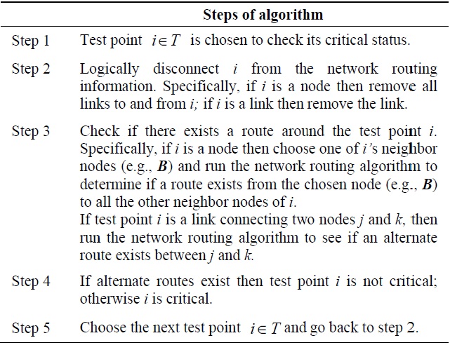
Here, we propose a new heuristic algorithm to identify topological critical points. Our proposed algorithm utilizes the network layer routing protocol to examine the alternate connectivity between neighbor nodes to identify critical points. The algorithm can be executed locally at a node as a self-test. The basic idea is to test a link or node for criticality by deleting all routes through the test point and seeing if alternate routes exist between neighbor nodes of the test point. If the test point is a link, alternate routes between the two end nodes are considered. Our proposed algorithm is shown below in Table 3.

The concept of the critical point identification algorithm is illustrated by example for the network of Fig. 2. Consider the test point node E, which has three neighbor nodes, B_e = {D, F, H}. The combinations of neighbor node pairs is given by, (D, H), (D, F), and (F, H). One can see from the figure that the neighbor node pairs all have an alternate path that does not go through node E. Hence node E is not a critical node. In contrast, consider node M as the test point node. Node M has four neighbor nodes, N, L, O, and P.

Note, that the neighbor node pairs (N, L) and (O, P) have an alternate path between them (i.e., N-I-J-K-L for N and L, O-P for O and P). However, nodes (O, N), ((O, L), (P, N), and (P, L) do not have an alternate path; thus node M is a critical node.

The time complexity of the proposed algorithm is largely determined by computational time to determine the routes between neighbor nodes. In fact, the proposed algorithm takes the same time as the routing algorithms adopted in the network.

Multiple critical points are a combination of nodes and/or links whose simultaneous failure partitions the network. For example, double critical nodes are a combination of two nodes/links whose failure causes the network to partition. Multiple critical points can be found by our proposed algorithm with modification of the test points. Consider the double critical node case, in which all combinations of two neighbor nodes, one neighbor node from one test point node and one neighbor node from another test point node, should be tested for alternate paths that do not include the test point nodes. If any combination of two neighbor nodes does nott have an alternate path, then the e test point nodes are double critical nodes. In determining double critical nodes, single critical nodes are excluded because the failure of any combination with a single critical node partitions the network. In Fig. 2, for example, the failure of any combination of nodes with node M partitions the network because node M is already a s single critical node. Node F and J are not single critical nodes and could be tested for double critical node status. the neighbor pairs of F and J, which are (A, H), (A, I), (A, K), (G, I), (G, H), (G, K), (E, I)), (E, H), and (E, K)), are considered for alternate paths with F and J removed. In this case, the node pairs (A, H), (G, I), (G, K), and (E, H) have alternate paths while other pairs off nodes do not. Thus, the combination of F and J form a double critical node pair.

Our proposed critical point test algorithm can also be used for local H-hop critical point identification as in [12]. Specifically, one uses the algorithm with all of the possible H-hop paths through each neighbor node of the test point. These alternate H-hop paths can be found at each node using receiving flooding messages that include visited node information. In the collection phase, all nodes send out a hello message adjusting the TTL value of H. Each node receives the hello message from all nodes within an H-hop. All intermediate nodes can easily insert their information by piggybacking on the hello message. Multiple hello messages may come from the same source where only one hello message arrives if only one path exists in an H-hop sub­network. For example in the network of Fig. 2, considering H = 3, node E receive s one hello message from node F, D, H, G, J, A, C, and K because those nodes are less than 3 hops away from node E and any alternate path has more than 3 hops in Fig. 2. From those nodes that have alternate paths In the H-hop sub-network around the test point node, more than one hello message will arrive through an alternate path. In Fig. 2, node E will receive 2 hello messages from node I (i.e., I-G-F-E and I-J-H-E) and another 2 hello messages from node B (i.e., B-A-F-E and B-C-D-E). The H-hop connectivity of node E in H = 2 and 3 are shown in Fig. 3.

Once a test point node collects H-hop sub-network connectivity information, it can determine its criticality status by testing alternate connectivity between neighbor nodes. Alternate connectivity can be determined by examining the sets of intermediate nodes of all pairs of neighbor nodes. If at least one common node exists, two neighbor nodes have alternate connectivity besides the route through the test point node.

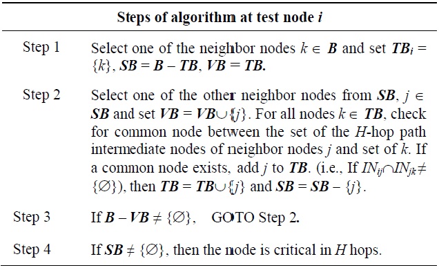
Each nodes checks the connectivity between all pairs off nodes from its neighbor nodes set B (i.e., B = {B_i; i = 1, 2, 3, …, d} where d is the node degree). If any neighbor node is not connected to other neighbor nodes in a direct or multi-hop fashion, the test point node is a critical node. Table 4 illustrates an algorithm to identify the local H-hop critical node.

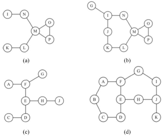
Consider the critical point identification problem using H-hop local connectivity regarding node M or E in the network topology of Fig. 2. The 2-hop and 3-hop connectivity sub-networks of node M are in Fig. 3(a) and (b), respectively. Similarly, Fig. 3(c) and (d) show 2-hop and 3-hop sub-networks of node E, respectively. In order to apply the critical point test algorithm, each test point M or E should examine all hello messages with a TTL value of 2. For example, node M in Fig. 3(a) will receive hello messages from I,K,P, and O via its neighbor node such as through I-N-M, K-L-M, N-M, L-M, P-M, P-G-M, G-M, and G-P-M. From those messages (i.e., P-M, P-G-M, G-M, and G-P-M), node M can find that neighbor nodes G and P have alternate routes, but that there are one between (N,L), (N,O), (N,P), (L,O), and (L, P). Therefore, node M determines that it is a local critical point in a 2-hop sub-network around it. Similarly, Fig. 3(b) and (c) s show that node M and E are local critical points in 3-hop and 2-hop sub-networks, respectively. However, the 3-hop sub-network of node E indicates that node E is not a local critical point due to 3-hop paths (i.e., B -A-F-E, B-C-D-E, I-G-F-E, and I-J-H-E); neighbor node D is connected to F via D-C-B-A-F, while F is connected to H via F-G-I-J-H. These results imply that false detection using an H-hop sub-network depends on the value of H. In general, for any localized test, if only local H-hop connectivity information is known, false positives on critical nodes or links will occur when the alternate routes are longer than the H-hop limit. It is worth noting that hop count limits on routes are often used in networks for performance reasons (e.g., end-to-end delay bounds).

We also observe that the set of global critical nodes will be contained in the set of all local critic al nodes identified by the algorithm with H-hop information. Hence, unlike the algorithms in [13], the critical test point algorithm will have a 100% global critical point detection rate.

In this section, we present two topology modification schemes to improve the resilience of the network by strengthening the connectivity around the critical node. The first scheme adds additional links to provide full connectivity around the critical node while the other scheme creates the minimum number of additional links in the H-hop sub-network to make the node no longer critical. The first scheme needs the connectivity information between neighbor nodes, while the other manipulates H-hop connectivity information. An assumption for both cases is that nodes have enough power to establish the required new links and for now we ignore interference issues and maximum power limitations.

1) Local Mesh Connectivity Scheme

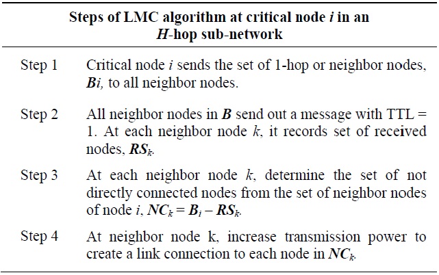
The local mesh connectivity (LMC) scheme creates a fully connected 1-hop local network around a critical node. An additional link between each pair of 1-hop nodes can be established by adjusting transmission power. All 1-hop nodes of the critical node check for direct link connectivity with all the rest of the 1-hop nodes or neighbor nodes set B of the critical node (i.e., B={B_i; i=1,2,3,…,d-1} where d is node degree). It can be determined by hello flooding message dissemination from the critical point identification process or new 1-hop messages. Then, it creates additional links to all other neighbor nodes, which have no direct link connectivity by increasing transmission power. The LMC algorithm is illustrated in Table 5.

Adding additional links between 1-hop nodes of the critical node creates an alternate path for each pair of 1-hop nodes so that the network is still connected even when the critical node fails. For example, node M is a critical node off the 3-hop sub-network in Fig. 3(b). Node MM, whose node degree is 4 (i.e., d_A= 4), has 4 1 -hop or neighbor nodes (i.e., B_M == {L, N, O, P}).

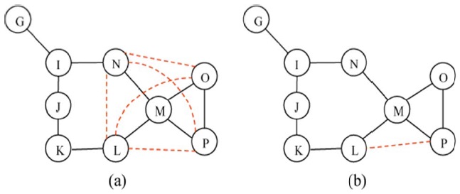
In the LMC scheme, all pairs s of neighbor nodes are to be examined for direct link connectivity (i.e., A(O,P)=1,,A(L,N)=A(L,O)=A(L,P)=A((N,O)=A(N,P)=0). Then, all nodes in all pairs of 1-hop or neighbor node shaving no direct link connectivity (i.e., LLN, LO, LP, NO, and NP) increase the transmission power until direct link connectivity is created between each other. As a result, a fully connected network is established around the critical nodes as shown in Fig. 4(a), where the dotted line represents the establishment of addition a links by adjusting the transmission power of each neighbor node. Then, node M is not a critical node anymore since there still exists connectivity between all pairs of neighbor nodes when node M fails. The number of nodes that increase their transmission power is 4, and 5 new links are created a round the critical node M in this example.

2) Local Least Connectivity Scheme

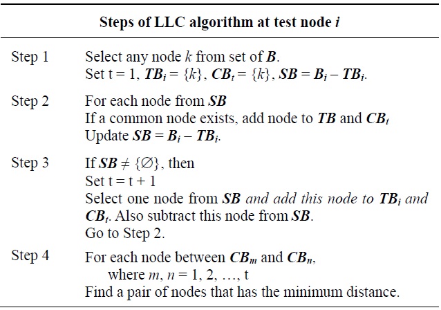
Similarly, the local least connectivity (LLC) scheme also creates additional links around a critical node. LLC finds fewer additional links than does LMC. Since LLC utilizes H-hop sub-network connectivity information, unnecessary links would not be created. In an H-hop sub-network, one or more alternate routes not including acriticalnodemayyexisstbetween 1-hop nodes of a critical node. Therefore, connected 1-hop nodes do not require an additional link, which reduces a number of meaningless additional links created by LMC. LLC also finds the minimum cost links between 1-hop nodes from each cluster, which also reduces the cost of creating an additional link. The LLC algorithm is illustrated in Table 6.

The example of LLC is shown in Fig. 4(b). Node M is a critical node and the sub-network breaks into two clusters when node M fails. 1-hop nodes L and N are connected via an alternate route (i.e., L-K-J-I-N) and they are in the same cluster, while the other 1-hop nodes O and P are directly connected. Then, LLC recognizes connectivity within the 3- hop sub-network and creates one additional link between L and P to create an alternate route between the two clusters assuming the distance L-P is shortest (i.e., dst(L,P) < dst(L,O), dst(N,O), dst(N,P)).

3) Implementation of the Schemes

The critical node initiates LMC and 1-hop neighbor nodes execute it. First, the critical node sends an initiation message including the set of 1-hop neighbor nodes to all other 1-hop nodes. As soon as this message arrives at each neighbor node, each 1-hop neighbor node sends a message to all of the other 1-hop neighbor nodes by setting the time-to-live (TTL) value of 1 to check for direct link connectivity. Only directly connected 1-hop nodes receive this message. Then, each 1-hop neighbor node learns which other nodes with which it should create an additional link.

Unlike in LMC, the critical node initiates and executes the LLC scheme. LLC uses the H-hop sub-network, which can be obtained from the H-hop critical node identification process. The information about all possible H-hop paths through 1-hop neighbor nodes from flooding messages informs the critical node of the set of visited nodes in all possible H-hop paths through neighbor nodes. The critical node can compare the visited node sets of each pair of neighbor nodes to determine the multi-hop connectivity. Thus, the critical node can identify connected and not connected 1-hop neighbor nodes within H hops. LLC then determines the minimum number of pairs of nodes needing an additional least cost link until each pair of clusters is connected. Note that the least cost links can be computed by acquisition of the node position utilizing global positioning system or localization techniques [13,17].

In this section, we present results from sets of simulations. We first present the numerical study of H-hop effects on critical node detection. Then, we present numerical results on the effect of the topology control resilient scheme in H hops on network parameters. The improvement in resilience by proposing resilient schemes is also studied.

We use our proposed critical point identification algorithm to illustrate the effects of limited information (i.e., H-hop) on critical node detection. At each node, it performs the critical point identification algorithm based on obtained H-hop sub-network information. This was implemented in MATLAB. We randomly generate network topologies with different numbers of nodes (50, 75, 100) in a 1,500 m × 1,500 m network area. The nodes are randomly and independently distributed in the network area with the (x, y) coordinates determined according to two independent uniform [0-1500] random variables. All nodes are identical and have a 250 m transmission range. For each node density, we randomly generate topologies until 100 connected topologies are found. For each network topology, each node finds H-hop connectivity in H = {2, 3, 4, 5} and executes the critical point identification algorithm to test for critical nodes. Fig. 5 shows the false detection rate of single and double critical node(s) using H-hop sub-network critical node(s). The false detection rate is calculated by dividing the number of falsely detected critical nodes by the total number of detected nodes by the H-hop critical point identification algorithm. As shown in Fig. 5, both the single and double false detection rates (i.e., FR1, FR2) are always lower with a larger H-hop since the larger H-hop subnetwork provides more accurate network connectivity information. The double critical nodes are a pair of nodes that partition the network when they fail at the same time. Similarly, FR also increases, as the network is denser. This is because limited H-hop connectivity information is less accurate in a denser network.

Comparing FR1 and FR2, critical node detection by an H-hop sub-network is more significant in double critical node identification. The falsely detected node for a signal critical node can be one of double critical nodes. For example, node F in Fig. 2 is detected as a critical node in a 2-hop sub-network, which is not a single critical node but one of double critical nodes (i.e., (F,E), (F,H), and (F,J)). Thus, FR2 is always lower than FR1.

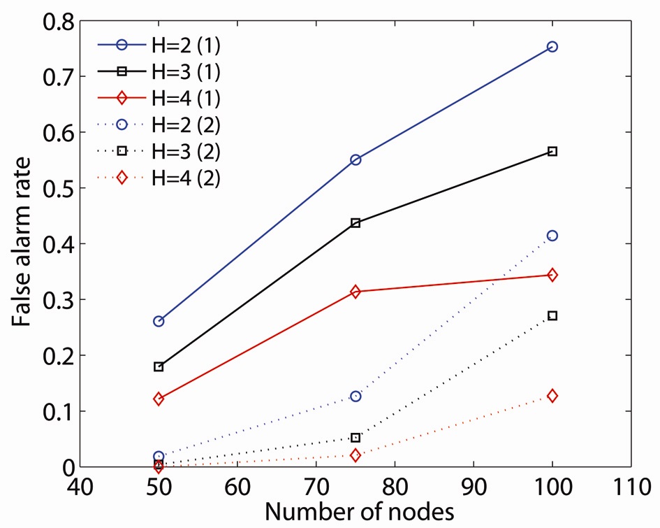
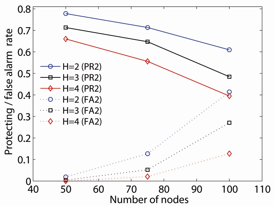
To illustrate the effect on double critical node detection, we introduce the protection rate of double critical nodes (PR2): the ratio of the number of double critical nodes in which at least one node is detected by an H-hop critical node to the total number of critical nodes. If either one of the double critical nodes is strengthened by the resilient scheme, the network remains connected at simultaneous failures of double critical nodes. Fig. 6 shows PR2 and FR2 in different H-hop values of 2, 3, and 4. Given that they have a lower H value for the H-hop, both PR2 and FR2 increase overall network density. FR2 does not show a difference by H-hop in a sparse network (i.e., FR2 = 0.0187, 0.00412, 0 at H = 2, 3, 4, respectively). FR2 increases dramatically with network density at a lower H value (i.e., FR2 = 0.0187, 0.1265, 0.4141 in 50, 75, 100 nodes density at H = 2). On the other hand, PR2 decreases, as the network is denser at all H values.

The value of the H-hop local critical node approach can be determined by the difference between PR2 and FR2. The difference between PR2 and FR2 is more significant in sparse networks and less significant in denser networks (i.e., PR2 ？ FR2 = 0.7592, 0.5869, 0.1953 in 50, 75, 100 nodes network at H = 2).

We evaluate the effectiveness of our critical node management schemes using simulation. In this study, we implement our proposed resilient schemes for H-hop local critical nodes and global critical nodes and then compare them. We generate random topologies with different numbers of nodes (i.e., 50, 75, and 100) in a network area of 1,500 m × 1,500 m. The nodes are independently distributed according to a uniform [0-1500] random variable in the network area. For each network density, we generate 50 connected random topologies, where every pair of nodes has at least one route (i.e., they are k = 1 or more connected) and at least one critical node in the topology. A free space propagation model is used and a uniform disk of the transmission range is created in the simulation. We assume all nodes are identical and have a capability of adjusting transmission power with an initial power with a transmission range of 250 m. We use MATLAB to implement our proposed critical node management schemes (LMC, LLC) at H = 2, 3, 4. First, we examine the effectiveness of the proposed schemes in providing k = 2 connectivity for the entire network. It makes 100% of 2- conneted networks for both schemes in 50, 75, and 100 nodes.

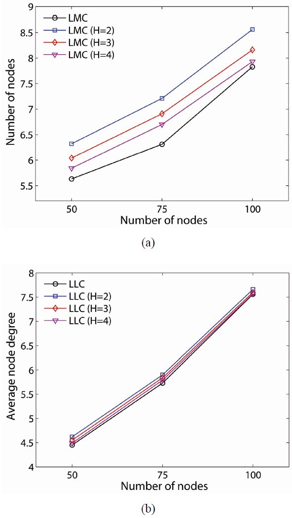
Although our proposed schemes can effectively provide a 2-connected network, there are some tradeoffs between LMC and LLC. We consider the average node degree and average number of added links as the tradeoffs, and they are shown in Figs. 7 and 8, respectively. The average node degree provides a metric of connectivity and interference. In the sparse network case (i.e., 50-node network), LMC has a higher average node degree (i.e., LLC 4.45, LMC 5.63). When the network is denser, the average node degrees of the proposed resilient schemes are closer. A different value for H in LLC does not make much difference in the average node degrees in all network density while LMC makes a difference. LLC on a global critical node shows a lesser average node degree than that on H-hop local critical nodes in 50-, 75-, and 100-node networks for all values of H (i.e., 5.63 global, 5.84 H=4, 6.04 H=3, 6.35 H=2, 6.35 at 50 nodes).

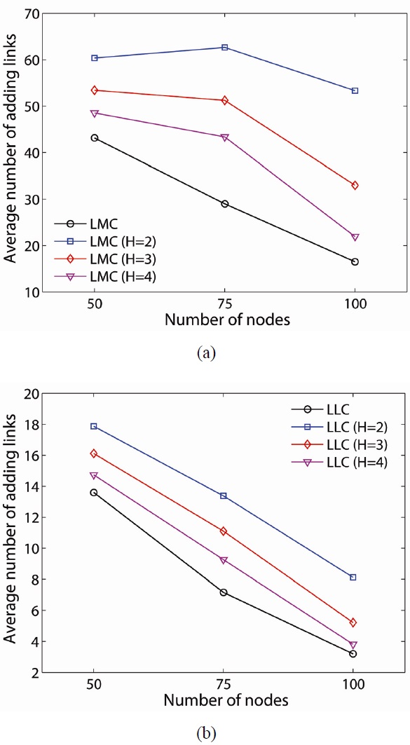
The average number of added links can be related to the average energy consumption of the network since adding additional links is achieved by increasing the transmission power of the node. As shown in Fig. 8, LMC requires significantly more energy than LLC for the 50-node network (i.e., 60.36 at H = 2) case since it requires a larger number of additional links. As network density increases, LMC still creates more additional links than LLC, but it is not as significantly large as it is in a 50-node network. A lower H-hop requires a larger number of added links for both LMC and LLC as expected. As the network density increases, the number of links decreases significantly except for LMC with H = 2 (i.e., 60.36, 62.64, 53.32 at 50, 75, 100 nodes, respectively).

To further examine the resilience of the proposed schemes, we randomly fail nodes and links in the network and determine the probability the network remains connected (i.e., P(Connected)). Each node fails according to probability P_nf, and each link with link failure probability P_lf. The probability of node failure was set to result in an average of one node failure for each network density (i.e., P_nf = 1/N). The link failure rate was varied (P_lf = 0.00, 0.05, 0.1, 0.15, 0.2), where P_lf = 0.1 means that on average 100 × P_lf = 10% of the links fail in the network. For each of the 50 topologies, we randomly generate 100 experiments for each P_nf and P_lf and determine the probability the network is connected.

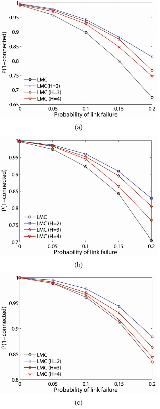
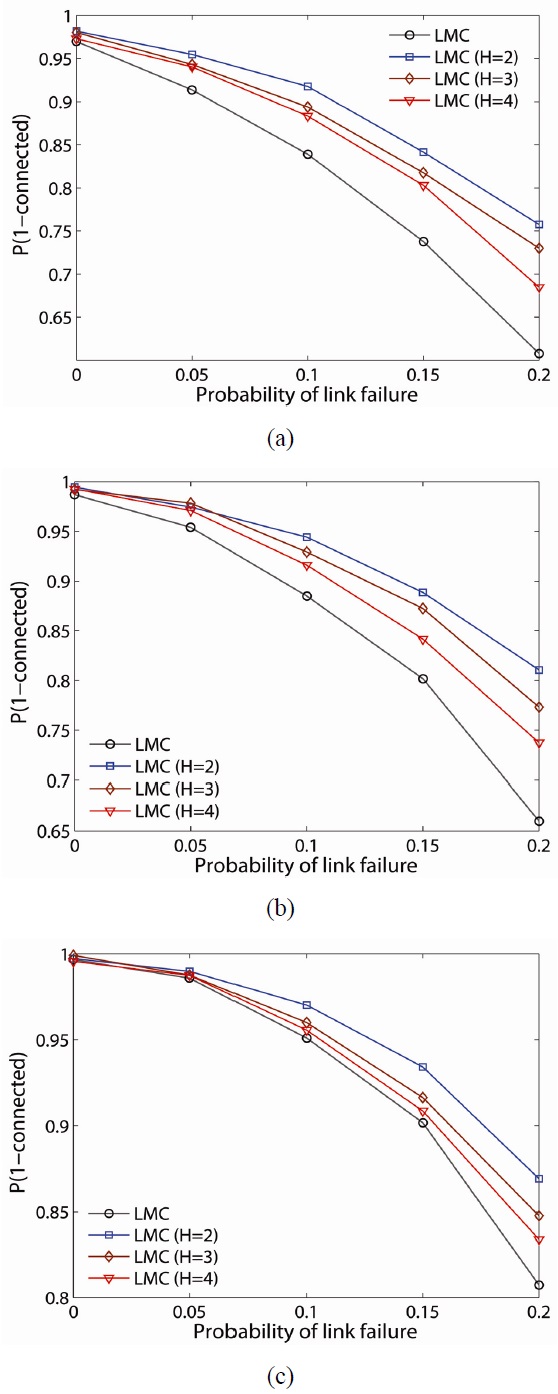
The probability of the network being connected on the estimate of LMC is computed and plotted for 50-, 75-, and 100-node networks, as shown in Fig. 9(a)？(c), respectively. As one would expect, the lower H-hop improves P(Connected) the most. For example, for the 50 node network case, the LMC scheme provides close to 95% chance the network is connected even with P_nf = 0.02 and P_lf = 0.1 at H = 2. As the network density increases, P(Connected) increases.

For example, for a 100-node network with link failure of 0.2, P(Connected) becomes 0.8348 by LMC on global critical nodes while LMC on H = 2 improves it up to 0.8838 and on H = 4 improves it to 0.8444 for the minimum improvement.

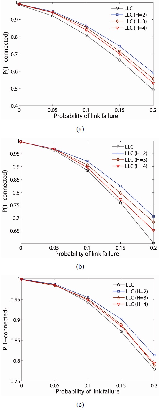
The probability, P(Connected), of LLC for 50-, 75-, and 100-node networks is shown in Fig. 10(a)？(c), respectively. As in LMC, LLC improves P(Connected) the most when implemented for a lower value of H (i.e., 0.8642 H = 2, 0.8554 H = 3, 0.8410 H = 4, 0.81 on global) with P_lf = 0.1 in a 50-node network. Similarly, LLC also provides a higher P(Connected) in a denser network. For example, for a 100- node network with a link failure of 0.2, P(Connected) becomes 0.7792 by LMC on global critical nodes while LFC on H = 2 improves it up to 0.8136 and on H = 4 improves it to 0.7942 for the minimum improvement.

When LLC is compared with LMC, LMC improves the probability of network connectivity more than LLC at any network density. Another observation is that P(Connected) decreases faster when implemented on global critical nodes as the network is experiencing more severe link failure. For example, in the 50-node network case, when the link failure rate increases from 0 to 0.2, P(Connected) decreases from 0.9922 to 0.6734 with global critical nodes while it decreases from 0.9968 to 0.814 with 2-hop local critical nodes (at H = 4, it shows the largest decrease in P(Connected) among H-hop local critical nodes ).

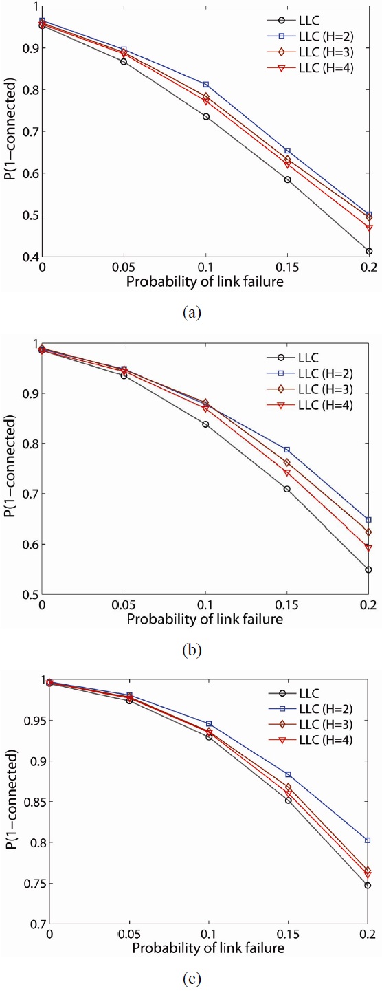
Figs. 11 and 12 illustrate P(Connected) of LMC and LLC with higher probability of node failure at each given link failure (i.e., P_lf = 0.00, 0.05, 0.1, 0.15, 0.2). In this set of studies, we used the probability of node failure, set to result in an average of two node failures for each network density (i.e., P_nf = 2/N). In more severe node failures, the results are similar to the results from the previous case (i.e., P_nf = 1/N). LMC has a greater probability of providing a 2-connected network than LLC. P(Connected) increases as the network is denser in both schemes. Similarly, the lower H-hop has a greater P(Connected) in both schemes. Note that the P(Connected) by LLC gets significantly lower at severe node and link failure as the network is sparser (i.e., 0.4124 on global for the minimum, 0.5004 at H = 2 for the maximum).

Note that while the LMC scheme has a higher P(Connected) under node and link failure, it consumes more energy. Thus it will be the best scheme in a sparse network if the network has unlimited or rechargeable power sources. Otherwise, either the LLC scheme is better because they create significantly less node interference and require less energy consumption than LMC. Both schemes on lower H-hop provide better connectivity but also create more interference and consume more energy. However, LMC will outperform in a sparse network with severe node and link failure conditions.

We have proposed a new algorithm to identify the critical connectivity points of a multi-hop wireless network topology utilizing the connectivity between local neighbor nodes. Unlike the existing algorithms, the proposed technique can be tested locally at the node and has a simple implementation using only local information at the expense of false positives in the results. Local sub-network critical nodes can be used to predict multiple failure critical points and can reduce the number of broadcasting messages by limiting the TTL value. We have also proposed two resilient schemes that strengthen the critical nodes by utilizing transmission power control. Our proposed schemes can be applied to global and local H-hop critical nodes and create a 2-connectivity network topology. The simulation results in a variety of node and link failure scenarios indicate that the proposed resilient schemes on local H-hop sub-network critical nodes outperform those schemes on global critical nodes in all network densities where a lower H-hop provides better connectivity. Furthermore, the LLC scheme on an H-hop local critical node is considered the best approach for improving the network resilience while minimizing energy and interference. Future research will focus on the prediction of critical nodes in an H-hop local sub-network approach. Since the network topology may change in time due to node mobility and interference, one should predict the critical points in advance.