The Light Aircraft Development Program is an initiative sponsored by the Korean Ministry of Land, Infrastructure and Transport Affairs. The project aims to enhance aircraft design, manufacturing, and certification expertise in the public sector. KLA-100 aircraft development program was performed by Konkuk University and 12 Organizations. The program was established in November, 2010 and will conclude in 2014 with the delivery of four prototype aircraft in the Very Light Aircraft (VLA) category [1]. Very Light Aircraft (VLA) category was aeroplanes category with a single engine (spark or compression-ignition) having not more than two seats, with a Maximum Certificated Take-off Weight of not more than 750 kg and a stalling speed in the landing configuration of not more than 83 km/h (45 knots).
The conceptual and preliminary design phases were allocated to the newly established Korea Aerospace Design, Airworthiness Institute (KADA) at Konkuk University in Seoul [1]. This has offered a unique opportunity to the Aerospace Engineering faculty and students, many of whom are contributing to the development of the aircraft. The detailed design phase as well as the manufacturing will take place at DACC Aerospace, an aerospace composite materials manufacturing company. DACC’s business is divided into main areas. They are carbon composites which are suitable for use in temperatures up 3,000℃ and lightweight structures, which are stronger then stell byt lighter then aluminum. The conceptual and preliminary design phases have been completed, resulting in the KLA-100 aircraft concept. The KLA-100 is a two-seat, low wing VLA aircraft with a 620 kg maximum takeoff weight powered by a 100 hp Rotax engine [1]. It is designed for short field performance and a long cruise range.
The conceptual design of light aircraft is typically carried out by using simplified analysis methods and empirical equations in a time consuming, iterative process. Recently, new conceptual design approaches have been proposed that harness computational design optimization methods to reduce time and effort required for the conceptual design while improving the result. Various analysis tools for modeling aerodynamics, weight, stability, and other disciplines are linked in a unified framework. Optimum conceptual designs are obtained by running one of the many widely available optimization algorithms. This approach has been shown to be effective in many case studies in recent literature. However, adoption of these techniques to support real design efforts is virtually non-existent in the light aircraft industry.
The research addresses several issues that arise during the conceptual design phase. Firstly, the reliability of the aircraft weight, drag, and performance analysis methods available early in the design process may be limited. Secondly, aircraft design goals and certification requirements such as stability, stall speed, range, and others need to be considered early in the design process. This paper outlines how these methods can be successfully implemented to support the development of light aircraft. A sophisticated multidisciplinary light aircraft design and optimization program was developed and used extensively in the conceptual and preliminary design stage of the KLA-100, a new Very Light Aircraft (VLA) currently under development.
The resulting concept continued to satisfy all of the initial requirements when validated using Computational Fluid Dynamics (CFD) and wind tunnel testing. This paper is aimed at investigating the satisfying of the resulting concept scheme by Computational Fluid Dynamics (CFD) works. There will be discretization study to the CFD implementation to prove whether the condition reasonable or not compare to wind tunnel testing. As such it should be able to handle a variety of geometries and to predict the aerodynamic effects of the full body configuration to a reasonable degree of accuracy, while achieving the low computational cost and time needed in design studies. This study considers the manufacturing tolerance effect to the surface area also.
In order to conduct the above mentioned research, a clean model configuration should be taken into consideration. It should be noted that the interaction of flow with the surfaces in computational, as well as the wind tunnel condition. In that respect, the paper will focus only on the aerodynamic effects of the surfaces. This research will serve as a first step towards the understanding and modeling of possible full body Very Light Aircraft computational works.
In order to define the scope and setup of the research, a formal objective is formulated. Following the definition of the main objective, a plan can be outlined on how to tackle it and how to structure the study that needs to be performed. The following section explains the objectives of this paper.
The main objective of this paper can be formulated as follows:
Investigate the effect of discretization studies of the full body Very Light Aircraft configuration on the aerodynamics characteristic of a low speed by means of numerical model and comparing to wind tunnel test.
The secondary objectives defining the scope of the project are summarized below:
Studying a tool capable of predicting the aerodynamic effects of full body aircraft configuration
Establish a range of applicability for the numerical tool
Employing the solver study and grid convergence study to get the optimum solver and mesh elements for the VLA model analysis
Focus on a surface discrete studies with the VLA manufacturing tolerance baseline in order to get the reasonable results compare to wind tunnel data
The numerical tool will consist of a full body aircraft model, combined with an existing design tool, called
Aircraft design begins with the conceptual phase, where possible designs are first imagined and evaluated from initial design requirements. In this phase, the designer has the greatest flexibility in determining the layout and configuration of the aircraft. After the conceptual phase, however, only minor changes to the aircraft configuration may occur. Therefore, it is important to have accurate drag and lift predictions early in the design phase when major configuration changes can occur. The accuracy of these predictions must be balanced, however, with calculation speed. This is needed so many types of configurations can be compared and so size optimization on a selected configuration may occur.
Aerodynamics for conceptual designs is typically based on linear aerodynamic theory, supplemented with empirical data. These methods work well for subsonic flows, where nonlinearities in the flow are negligible, but break down when the nonlinearities become important. For flows that are entirely supersonic there are nonlinear methods that work well for aerodynamic predictions. However, for transonic flows these methods fail because the flow has both subsonic and supersonic areas. The desire for more accurate lift and drag prediction for transonic flows-along with a more detailed analysis of the flow field for all flows types have resulted in the increased use of Computational Fluid Dynamics (CFD) early in the design stage.
Computational fluid dynamics (CFD) has developed into a valuable design tool. It is now possible to compute the flow around complex aerospace configurations such as complete aircraft, helicopter and spacecraft [2]. This rapid increase in CFD applications over the last few decades has become possible by ever increasing computer power, more efficient numerical algorithms and progress in physical modelling.
2.2.1 Grid Convergence Study
The examination of the spatial convergence of a simulation is a straight-forward method for determining the ordered discretization error in a CFD simulation. The method involves performing the simulation on two or more successively finer grids. The term
Methods for examining the spatial and temporal convergence of CFD simulations are presented in the book by Roache [4]. They are based on use of Richardson's extrapolation. A general discussion of errors in CFD computations is available for background. We will mostly likely want to determine the error band for the engineering quantities obtained from the finest grid solution. However, if the CFD simulations are part of a design study that may require tens or hundreds of simulations, we may want to use one of the coarser grids. Thus we may also want to be able to determine the error on the coarser grid.
The easiest approach for generating the series of grids is to generate a grid with what one would consider
2.2.2 Surface Tolerance Study
In Autodesk Simulation CFD, the finite element method is used to reduce the governing partial differential equations (PDEs) to a set of algebraic equations [5]. In this method, the dependent variables are represented by polynomial shape functions over a small area or volume (element) [5]. These representations are substituted into the governing PDEs and then the weighted integral of these equations over the element is taken where the weight function is chosen to be the same as the shape function [5]. The result is a set of algebraic equations for the dependent variable at discrete points or nodes on every element. This paper is, therefore, devoted to enhancing the calculation time; there will be a several study in discrete points or nodes on every element surface as a surface treatment with the automatic surface mesh element control. That scheme will use the VLA tolerance zone as a baseline.
Design automation with finite element analysis as a simulation and evaluation tool is becoming more and more desired. The ability to do automatic design iteration has constantly been a popular research and engineering topic. Parametric modeling is crucial and necessary for numerical design optimization. However, being able to do parametric modeling does not mean you can use it for optimization. Numerical optimization does have its limitation and assumptions. Our experience has shown that blindly coupling a parametric model together with optimization routine will usually cause serious problems. This is why the above-stated methodology was developed.
ANSYS was one of the solver code that can figured out above parametric modeling and one of the famous design automation. ANSYS is a finite-element analysis package used widely in industry to simulate the response of a physical system to structural loading, and thermal and electromagnetic effects. ANSYS uses the finite-element method to solve the underlying governing equations and the
ANSYS renowned fluid analysis tools include the widely used and well-validated ANSYS FLUENT and ANSYS CFX, available separately or together in the ANSYS CFD bundle [6]. ANSYS FLUENT software contains the broad physical modeling capabilities needed to model flow, turbulence, heat transfer, and reactions for industrial applications ranging from air flow over an aircraft wing to combustion in a furnace, from bubble columns to oil platforms, from blood flow to semiconductor manufacturing, and from clean room design to wastewater treatment plants [6]. Special models that give the software the ability to model in-cylinder combustion, aeroacoustics, turbomachinery, and multiphase systems have served to broaden its reach [6].
This paper is, therefore, devoted to enhancing the calculation and work time efficiency, this master thesis will implement this ANSYS FLUENT numerical tools. Design automation and friendly user could be the one of the main purpose for choosing this numerical tools. The target for the accuracy was included in this software main purpose and it was fit with the purpose of this paper.
Designs using CFD were based on simplified physical models such as panel methods and linear theory. Where gradient-based optimisation algorithms were employed, aerodynamic sensitivity information was calculated using simple finite-difference techniques. This method of computing design sensitivities requires virtually no modification to the existing analysis code.
In this research, aerodynamic sensitivity is the main feature to be discussed. The importance of this research is with regard to how we manage calculation and sensitivity in a model. The purpose is to obtain accurate data to compare the real condition with the model. The goal is to determine how we attain the condition nearest to the real condition or experimental work. After we have the most accurate data, it can be used as a baseline reference for similar case models, which will be more effective in time and cost compared to experimental work.
In Murayama and Yamamoto computations were performed using two CFD codes based on different mesh systems (multi-block structured and unstructured mesh) in solving the flow field around a three-element (slat, main, and flap) trapezoidal wing with fuselage [6]. The aerodynamic forces were predicted reasonably, even with the unstructured mesh when moderate settings for the slat and flap were used [7].
Unstructured mesh methods for computational fluid dynamics have been under development for over 25 years [8]. The original attraction of this approach was based on the success achieved in handling complex geometries, as demonstrated through finite-element-based approaches, mainly in the field of structural analysis. In addition to the flexibility in dealing with complex geometries, the ability to easily incorporate adaptive mesh refinement (AMR) strategies also became one of the often quoted advantages of the unstructured mesh approach [8].
For this research, there is also a limitation for acquiring the reasonable data needed compared to experimental data. Computer performance and the unstructured scheme employed are our limitations in this study. There are two kinds of scheme, which are the main ideas for unstructured mesh generation to approach sensitivity in aerodynamic characteristics, besides other considerations. Every scheme employed contributes differently to reasonable results based on computer performance.
There are three main studies in this discretization scheme. Firstly we conduct the solver study validation. The solver study validation will figure out the effective solver for the KLA 100 model analysis. The second step was the grid element convergence validation. This step performs the optimum element analysis that will use for the next step study validation. The third study was about the surface tolerance study validation. This final study will perform the densities in several important area regarding to the manufacturing tolerance zone set.
Because of rapid advances in computer speeds and improvements in flow-solvers, a renewed emphasis has been placed on extending computational fluid dynamics (CFD) beyond its traditional role as an analysis tool to design optimisation. The governing equations are
The fundamental basis of fluid dynamics is the Navier- Stokes equations. In this study,
At high Reynolds numbers the rate of dissipation ε of kinetic energy is equal to the viscosity multiplied by the fluctuating vortices. An exact transport equation for the fluctuating vortices, and thus the dissipation rate, can be derived from the Navier-Stokes equation. The k-epsilon model consists of the turbulent kinetic energy equation and the dissipation rate equation.
4.3 Discretization Study Validation
4.3.1 Solver study validation
In order to make effectiveness in validation work, it is good to implement simple 2D and 3D model with the similar condition and characteristic with the KLA 100 model. These advantages refer to time and cost effectiveness in time calculation. The validation study for several model of 2D and 3D model are for default solver in computational calculation. It will be more effective if we employ the similar condition to simple model than the complex geometry of the master thesis model required. The main purpose for this validation study is to minimize the time to find the most effective solver for the KLA-100 model.
4.3.1.1 NACA 64(2)-415 validation
Validation study for this kind of airfoil is quite good. The type of the airfoil used in KLA-100 wing model was similar with this NACA 64(2)-415. It is important to carry out this study, because wing is the most important area for the
aerodynamic phenomenon occurs. For this implementation study, hopefully we can get at least the solver for the phenomena on the wing surface.
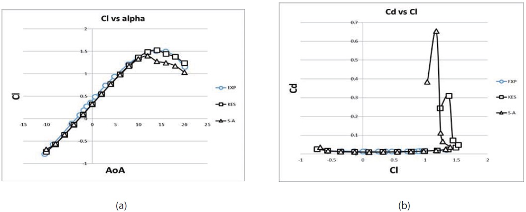
Initial condition for this calculation is according to experiment condition from the book of Theory of Wing Sections [9]. For the subsonic condition and sealevel condition, the 3.1x10⁶ Reynolds number is the fit condition for analysis. The results analysis of NACA 64(2)- 415 was figured as table 2. K-epsilon and Spalart-Allmaras turbulent model will employed to these solver validation works.
K-epsilon and Spalart-Allmaras turbulent model is a low-cost RANS model solving a transport equation for a modified eddy viscosity [10]. It designed specifically for aerospace applications involving wall-bounded flows. They are the most widely-used engineering turbulence model for industrial applications [10]. Those are some consideration for choosing the two kind of turbulent models as validation work. Those are very effective not only in cost and time but also in general users work implementation.
The computational condition was using unstructured
[Table 1.] Initial condition for the NACA 64(2)-415
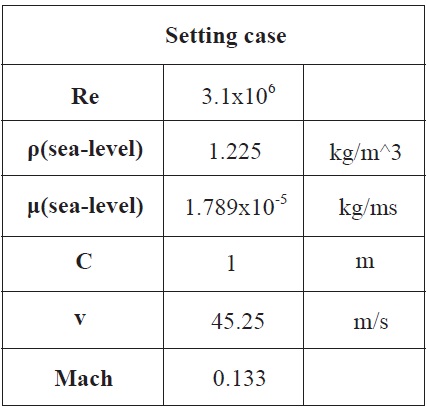
Initial condition for the NACA 64(2)-415
mesh with 180,000 mesh elements. The maximum coefficient lift error difference compared to experiment data is about 0.0195. It is quiet good to reach the stall condition with the K-Epsilon turbulent model. It can reach the stall area characteristic than Spalart-Allmaras model. For the computational work time, this paper will employ the unstructured scheme for the calculation. It is better for the complex configuration like KLA-100 model. As the comparison, we can see the table result and the graph for the aerodynamic data using K-Epsilon model compare to the experiment data provided in figure 1 and table 2.
For this 2D airfoil validation analysis, we can get the optimum turbulent model for reasonable aerodynamic characteristic approaching is K-Epsilon model. The unstructured mesh scheme is quiet good also to implement for the model.
4.3.1.2 ONERA M6 wing validation
This case involves the flow over the ONERA M6 wing.
[Table 2.] (a) Aerodynamic Computational results (b) Experiment data for NACA 64(2)-415

(a) Aerodynamic Computational results (b) Experiment data for NACA 64(2)-415
[Table 3.] Flow conditions for Test 2308 of Ref. 1. [11]

Flow conditions for Test 2308 of Ref. 1. [11]
It was tested in a wind tunnel at transonic Mach numbers (0.7, 0.84, 0.88, 0.92) and various angles-of-attack up to 6 degrees. The Reynolds numbers were about 12 million based on the mean aerodynamic chord. The wind tunnel tests are documented by Schmitt and Charpin in the AGARD Report AR-138 published in 1979.
The Onera M6 wing is a classic CFD validation case for external flows because of its simple geometry combined with complexities of transonic flow (i.e. local supersonic flow, shocks, and turbulent boundary layers separation) [11]. It has almost become a standard for CFD codes because of its inclusion as a validation case in numerous CFD papers over the years. In the proceedings of a single conference, the 14th AIAA CFD Conference (1999), the Onera M6 wing was included in 10 of the approximately 130 papers [11].
Currently, the CFD simulations use the flow field conditions of Test 2308 of Reference 1. Table 3 lists these flow conditions. These correspond to a Reynolds number of 11.72 million based on the mean aerodynamic chord of 0.64607 meters.
The ONERA M6 wing is a swept, semi-span wing with no twist. It uses a symmetric airfoil using the ONERA D section. The coordinates below indicate that there is a finite thickness to the trailing edge. For CFD simulations, an approximation is usually made of a zero trailing edge thickness.
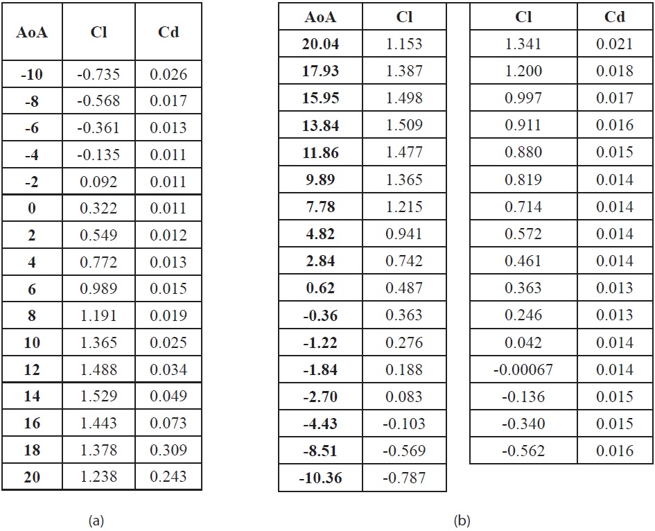
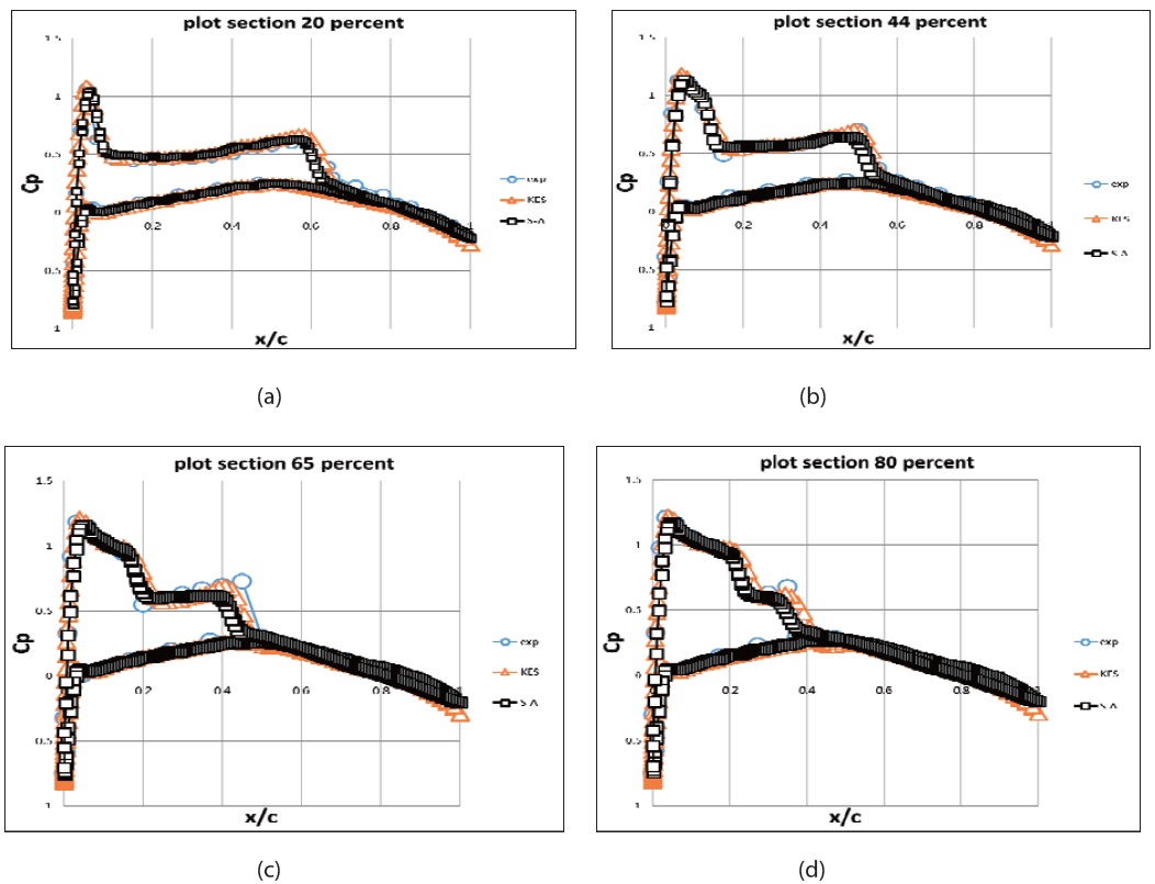
Comparison data consists of pressure coefficients at sections along the span of the wing obtained in the experiment performed by Schmitt and Charpin as data result figured below. These pressure coefficients are along the lower and upper surfaces of the wing at each of the four sections. The spanwise location of the sections are specified with respect to the wing span. The section location are 20, 44, 65, and 80 percent of wing span measured from the root.
Computational work for this Onera M6 wing was done with the K-epsilon and Spalart-Allmaras turbulent model implementation. With the unstructured scheme, the K-epsilon turbulent model can reach the most reasonable pressure coefficient compare to the experiment data than the Spalart-Allmaras model. The K-epsilon model catches the shock flow better than Spalart-Allmaras as figure 2 below. K-Epsilon turbulent model was a reasonable turbulent
solver also for the low speed condition in order to catch the aerodynamic characteristic. The unstructured scheme was also the reasonable scheme to implement to the KLA-100 model.
4.3.2 Grid Convergence Study validations
The configuration used in this study is a Very Light Aircraft (VLA) 3D full wing-body clean configuration. The fuselage length is 5.8 metres and the wing span is 9.5 metres. The volume is 3.63 m3. It has flap, aileron, horizontal stabiliser, vertical stabiliser, and rudder but only clean configuration was used for this present study. This VLA uses a propeller engine.
Mach number is 0.118 and the Reynolds number, Re, is 0.658x10⁶. In the computations, the flow was assumed to be fully turbulent. The temperature and pressure condition were set on sea level condition for all the cases. The temperature set as 288.16 K and the pressure set as 101,327 Pa. The outer boundary is located 50 chord lengths away from the airfoil. This mesh includes quadrangle elements around all fluid areas and triangular elements to fill all surfaces.
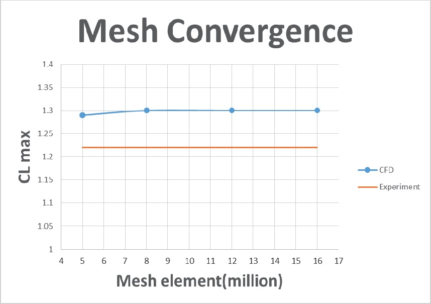
As the theoretical concept approaching, these convergence studies was done by the validation using several meshes elements. In figure 3, it is shown that the changes in the computed lift and drag coefficient decrease monotonically with an increasing grid resolution from 5 million meshes to 8 million meshes. The lift and drag coefficient from 8 million to 12 and 16 million are very similar.
The level of convergence for this large amount of mesh is
These convergence study done for accomplish the optimum mesh element to employ for the discretization study. This is kind of step work to do for discretization scheme. It is difficult to take one element of mesh randomly for discretization work, so that we can approach it with this convergence calculation. After we find the convergence point for this convergence study, it will be used for the baseline element mesh for discretization study.
[Table 4.] Computed data of CLmax and the Number of Grid Points with Experimental Data
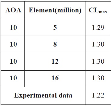
Computed data of CLmax and the Number of Grid Points with Experimental Data
The convergence level for the lower angle of attack reaches the 2000 iteration as figure above and the total time was 4.3 hours, 10 hours, 11.25 hours, and 48 hours respectively for 3, 8, 12, and 16 million mesh elements for one angle of attack. The convergence level satisfied in 10-4 for high angle of attack required in 3000 iteration and the total time was 6.5 hours, 15 hours, 17.10 hours, and 72 hours respectively for 3, 8, 12, and 16 million mesh elements for one angle of attack. If we calculate the total time for grid convergence study, for 8 angles of attack, it took 45.4 hours, 105 hours, 119.25 hours, and 504 hours respectively for 5, 8, 12, and 16 million mesh elements. This level of convergence was important for the smooth aerodynamic trend issue. For that issue, it is important to keep the level of satisfaction in every case calculation. With that condition, we can get the more reasonable result.
From Computed data of the maximum coefficient lift and the number of grid points with experimental data above, we can see the converged point of the maximum coefficient lift was around 1.30. Comparing to the CL from experiment data with 1.22, it was still reasonable although our purpose on this step study was for finding optimum point of element mesh. The continuous study hopefully did the more reasonable result for the validation.
4.3.3 Surface Tolerance study validations
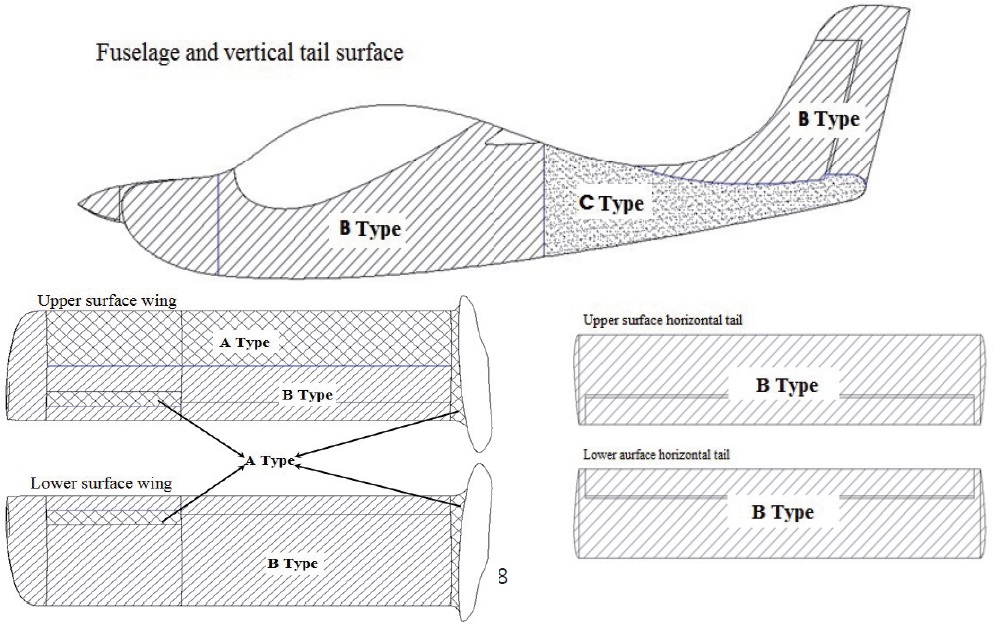
The tolerance zone of the outer surface set is considered in this grid discretization as a baseline. Zoning complies with the requirements that apply to the aircraft aerodynamics, depending on the importance, and is divided into the three areas described below:

A type: very important area for consideration of aerodynamic characteristics. Apply the mesh with very high tolerances.

B type: important area for consideration of aerodynamic characteristics. Apply the mesh with medium tolerances.

C type: average area for consideration of aerodynamic characteristics. Apply the mesh with low tolerances.
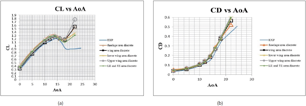
Computational works for all the scheme study are using unstructured mesh implementation. As the previous study in convergence study, we already got the optimum element mesh to use in discretization study. In this scheme, there will be several surfaces discrete to show which surface discrete type could be satisfied compare to experiment data.
According to the Prototype Manufacturing Tolerance Zone above as our baseline analysis for the surface discrete, there were 5 main type of area to be considered for surface discrete implementation. Those are wing area discrete, upper wing area discrete, lower wing area discrete, leading & trailing edge area discrete, and fuselage area discrete.
After the several step and study implemented, we have got the final result for the convergence and discretization study for the determination of the Very Light Aircraft (VLA) manufacturing tolerance as figured below. The results were the 8 million mesh elements with the wing, upper wing, lower wing, and TE &LE surface area discrete employed.
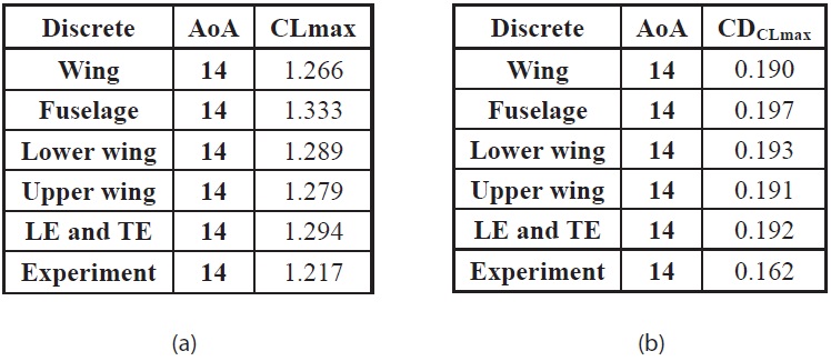
The unstructured mesh with tolerances for several surfaces can indicate the accuracy of the aerodynamic characteristics of the model. As shown in figure 5 and table 5, indicate that the aerodynamic characteristics was approach the required accuracy with a good tolerance on the wing surface. Calculating time for surface tolerance study validations was 105 hours in every discrete scheme. It was similar with the 8 million mesh elements time calculation from grid convergence study. It was similar because we use the same mesh element for this discrete scheme. The total time for all the discrete scheme was 525 hours.
5. Conclusions and Recommendations
In grid convergence study using the unstructured meshes, the 8 million element mesh was found to be the optimum mesh for the aerodynamic sensitivities of the KLA 100 configuration. Grid discretization study has been performed to investigate the time and cost effectiveness of the same size mesh with various local surface mesh densities.
Feasibility of the proposed process and the numerical results for this type of aircraft has been presented. The results of the grid discretization study confirmed that the current prototype manufacturing tolerance as our baseline was properly set in general. The lower wing surface tolerance should be equivalent to the upper wing surface tolerance. Wing surface is the main important area for consideration in order to achieve aerodynamic characteristic validation. The most feasibility study for this KLA-100 model was employing the K-epsilon standard turbulent model with 8 million mesh elements and with the wing area discrete implementation.
There will be several recommendations for future works regarding to this research. Those are kinds of advanced work
[Table 5.] (a) Maximum CL in every discrete scheme (b) CD data from the maximum CL

(a) Maximum CL in every discrete scheme (b) CD data from the maximum CL
to do for better achievement in this research fields. The future works can be explained as below.
1) Improved ways of grid density localization for grid discretization study.
2) More refined grid discretization study for aerodynamic sensitivities of the control surface.
3) Corresponding intensive aerodynamic analysis for KLA 100 configurations with the various deflection angles of the control surfaces such as flap, aileron, elevator, and rudder.
4) With this reasonable result, we can use these results for the Fluid Structure Interaction works for the aerodynamic data needed. Even in this future work there was a kind of issue to be considered about the both different target and consideration in mesh discretization from aerodynamic and structure works, it will be such an interesting topic research to continue in the next step study research.


![Flow conditions for Test 2308 of Ref. 1. [11]](http://oak.go.kr/repository/journal/12082/HGJHC0_2013_v14n2_122_t003.jpg)

![Prototype Manufacturing Tolerance Zone of the Outer Surface Set [12]](http://oak.go.kr/repository/journal/12082/HGJHC0_2013_v14n2_122_f004.jpg)