Intrusions can be defined as actions that attempt to bypass the security mechanisms of computer systems [1-3]. Intrusions may take many forms: attackers accessing a system through the Internet or insider attackers; authorized (official) users attempt-ing to gain and misuse non-authorized privileges. So, we say that intrusions are any set of actions that threaten the integrity, availability, or confidentiality of a network resource. Intrusion detection is the process of monitoring the events occurring in a computer system or network and analyzing them for signs of intrusions. Intrusion detection systems (IDS) raise the alarm when possible intrusions occur.
A lot of research into artificial neural networks (ANNs) has been undertaken. In [4], artificial neural networks and support vector machine (SVM) algorithms were applied to intrusion detection (ID), using a frequency-based encoding method, on the DARPA dataset. The authors use 250 attacks and 41,426 normal sessions and the detection rate (DR) varied from 100% to 43.6% with the false positive rate (FPR) ranging from 8.53% to 0.27% under different settings. In [5], the author concludes that the combination of a radial basis function (RBF) and self-organizing map (SOM) is useful as an intrusion detection model. He concludes that the “evaluation of human integration” is nec-essary to reduce classification errors. His experimental results showed that RBF-SOM achieves similar or even better results, compared to just an RBF. In [6], the authors use hierarchical (SOM) and conclude that the best performance is achieved using a two-layer SOM hierarchy, based on all 41-features in the KDD dataset and the ‘Protocol’ feature provides the basis for a switching parameter. The detector achieved an FPR and DR of 1.38% and 90.4% respectively. In [7], the authors use a hier-archical ID model using principal component analysis (PCA) neural network that gave a 97.1% DR and a 2.8% FPR. In [8], a critical study about the use of some neural networks (NNs) is used to detect and classify intrusions, the DR was 93.83% for the PCA approach, and the FPR was 6.16% for PCA. In [9], the authors present a biologically inspired computational approach to dynamically and adaptively learn signatures for network intrusion detection using a supervised learning classifier sys-tem. The classifier is an online and incremental parallel produc-tion rule-based system.
It should be noted that most of the previous systems concen-trate on either detecting two categories (normal or attack) or detecting a certain category of attack. Also all of the previous work ignores the symbolic features of the KDD Cup 1999 data set, this adversely affects the accuracy of detection. This study suggested a back-propagation neural network intrusion detec-tion system (BPNNIDS) and a radial basis function neural net-work intrusion detection system (RBFNNIDS). Both can perform either two category or multi-category detection and at the same time they do not ignore the symbolic features of the data.
This paper is organized as follows: Section II introduces the intrusion detection taxonomy, Section III explains the method-ology and the proposed system architecture, Section IV presents the experimental results and finally Section V concludes the paper.
II. INTRUSION DETECTION TAXONOMY
In short, intrusions are generally classified into several cate-gories [8]:
Attack types that are classified as:
○ Denial of service (DoS)
○ Probe (PRB)
○ Remote to login (R2L)
○ User to root (U2R)
Single network connections involved in attacks versus multiple network connections
Source of computer attacks:
○ Single attack versus multiple attacks
Network, host and wireless networks
Manual attacks and automated attacks
In short, IDS are generally classified according to several categories as follows [5, 7, 10]:
Work environments that can be classified as having host-based IDs or network-based IDs
Analysis that can be classified as anomaly detection or misuse detection.
Analysis that can be classified as real-time analysis or off-line analysis.
Architecture that can be classified as single and centralized or distributed and heterogeneous.
Activeness that can be classified as active reaction or pas-sive reaction.
Periodicity that can be classified as continuous analysis or periodic analysis.
The system proposed in this paper is considered to be net-work based, misuse with the ability to merge new attacks in one of the main four categories (DoS, PRB, U2R, and the R2L), offline and passive.
III. THE PROPOSED SYSTEM ARCHITECTURE
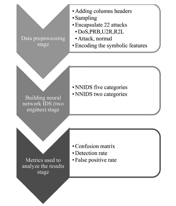
The proposed system architecture (Fig. 1) is primarily based on three stages: data pre-processing stage, building the neural network intrusion detection system (two engines) stage and metrics used to analyze the results stage. The three main stages of the proposed system architecture and their respective sub groupings are discussed in more detail in the following sections. According to a survey about the DARPA 98, KDD Cup 99 datasets, it should be noted that this dataset has been the target of the latest research [11, 12].
>
B. Data Pre-processing Stage
The data pre-processing stage consists of the following:
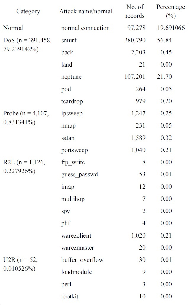
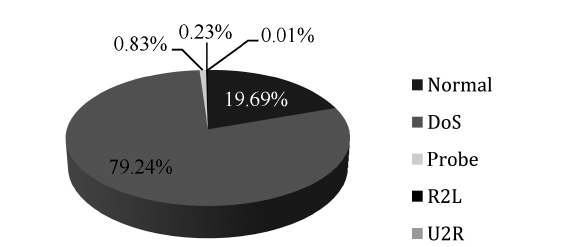
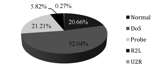
As we can see in Fig. 2, the DoS represents the majority of the dataset followed by the other normal connections, where the rest of the categories represent less than 1% of the training dataset. Thus the neural network model will be over trained in
[Table 1.] 10% version of the KDD Cup 1999 dataset distributions

10% version of the KDD Cup 1999 dataset distributions
the two major types, taking very long time in learning repeated data, at the same time it will consider minor types as noise due to their negligible percentages in the training dataset. To over-come this problem, the 10% version of the KDD Cup 1999 dataset is sampled in a way that the percentages of the various categories are of comparable value. The proposed system is trained using both the original and the sample dataset.
It should be noted from Table 1 that, we have only three records of high value: normal, smurf and neptune. This should be taking into consideration in the sampling process, i.e., only these values should be decreased.
An iterative reduction algorithm is proposed and applied to the (10% version of the KDD Cup 1999 dataset) as follows:
1. Search for the top-3 major values and consider them set S1.
2. The rest of the values are considered as set S2.
3. The maximum value of connection V1 in S2 is selected.
4. The values in S1 are reduced to be comparable to V1 and at the same time their order is maintained.
5. The performance of the system is tested with the new values.
6. Steps 4 and 5 are repeated until optimum results are obtained.
The original KDD Cup 1999 dataset can be divided easily into two categories. The first category (S1) consists of 3 attacks with a massive amount of available samples. The second cate-gory (S2) consists of the rest of the attacks; each of them is rep-resented with less than 1% of the dataset’s samples. This could make the system treat them as noise and not recognize them as separate classes. So, the reduction algorithm takes a portion of the dataset where all categories are represented by a percentage that cannot be neglected by the classification system while keeping their relative abundance.
Reducing the top 3 records should take into consideration the other category records (S2). The 3 records shouldn't be reduced to values less than the maximum of the other category records (S2). So the record with maximum number of samples must be identified (V1) such that V1 ? S2 where V1 = Max (S2).
The 3 chosen records (S1) will then be reduced iteratively keeping their values larger than V1 such that S1 (i) ≥ V1 where 1 ≤ I ≤ 3. Also the algorithm tries to maintain the order and pro-portion of the reduced records compared to the original dataset size especially the “normal” record to keep the false positive alarm rate as low as possible. After each iteration, the perfor-mance of the proposed system is measured using the new values generated by the algorithm.
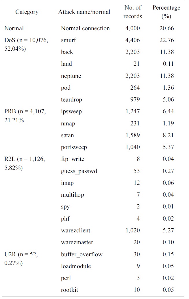
Optimum results are obtained when reducing the normal con-nections from 97,278 records to 4,000 records, the smurf records from 280,790 records to 4,406 and the Neptune records from 107,201 to 2203 as shown in Table 2.
Figs. 2 and 3 show the distributions of the normal and attack connections in the dataset before and after applying the pro-posed iterative reduction algorithm. Comparing these figures, it can be shown that the percentage of normal connections is approximately the same, this is important for reducing the FPR. The percentage of DoS records is reduced from 79% to 52% due to the reduction in smurf and neptune but it is still high compared to other categories. The percentages of both probe and R2L records have changed to significant values can now be seen in the dataset. This guarantees that the network will recog-nize these two types along with the other ones. Regarding the U2R category, this one is considered as host attack. This
[Table 2.] Our selected KDD Cup 1999 dataset distribution

Our selected KDD Cup 1999 dataset distribution
research focuses only on network attacks, where U2R is consid-ered as a noise in this research. The main advantage of this is reducing the training data from 494,021 records to 19,361 that greatly reduce straining time.
Finally, we will work using two datasets, a 10% version of the KDD Cup 1999 dataset and the proposed reduced dataset. We will compare the performance for both.
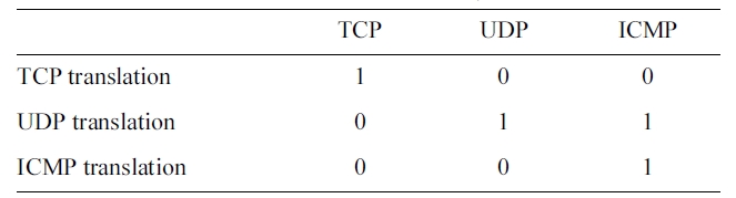
[Table 3.] Translation of the PROTOCOL_TYPE symbolic feature

Translation of the PROTOCOL_TYPE symbolic feature
[Table 4.] The KDD Corrected testing set

The KDD Corrected testing set
encapsulation are proposed. The first one is to encapsulate the 22 attack names to their four original categories DoS, PRB, R2L and U2L. The second one is to encapsulate the 22 attack names to the word attack.
We will work with two systems; the first one uses the first type of encapsulation and has five categories: DoS, PRB, R2L, U2L and normal. The second system uses the second type of encapsulation and has two categories: attack and normal.
As an example, the Encoding of the PROTOCOL_TYPE fea-ture is shown in Table 3. The rest of the symbolic features are translated in the same way.
>
C. Building Neural Network IDS Stage
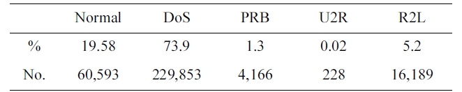
Two systems are built; the first is a system that consists of five categories: DoS, PRB, R2L, U2L and normal. The second one is a system that consists of two categories: attack and nor-mal. Two engines are used: back-propagation [13] and the radial basis function [14, 15]. The structure of the two systems will be explained in subsequent paragraphs. For the testing step, the KDD set was used (Table 4). The KDD corrected testing set contains 311,029 records, including records that describe 15 new attack types [16-19].
The algorithm can be summarized by the following steps [14, 15]:
1. Initialize the weights of the network (often randomly).
2. Present a training sample to the neural network where, in our case, each pattern x consists of 115 features after the translation of the symbolic features.
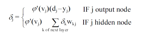
3. Compare the network's output to the desired output from that sample. Calculate the error for each output neuron.
4. For each neuron, calculate what the output should have been, and a scaling factor i.e. how much lower or higher the output must be adjusted to match the desired output. This is the local error.
5. Adjust the weights of each neuron to lower the local error.
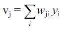
wji = wji + Δwji
With Δ
Δwji(n) = αΔwji(n - 1) + ηδj(n)yi(n)
For sigmoid activation functions
?' (vj) = ayj (1?yj)
where
with
to node
6. Repeat the process from step 3 on the neurons at the previ-ous level, using each one’s “blame” as its error.
Feed forward neural networks have complex error surfaces (e.g. plateaus, long valleys etc.) with no single minimum. Add-ing the momentum term is a simple approach to deal with this problem.
There are two types of network training: incremental mode and batch mode. In incremental mode (on-line or per-pattern training), the weights are updated after presenting each pattern.In batch mode (off-line or per-epoch training), the weights are updated after presenting all the patterns. In the proposed system we used the incremental mode.
For standard RBF’s, the supervised segment of the network only needs to produce a linear combination of the output at the unsupervised layer. Therefore having zero hidden layers is the default setting. Hidden Layers can be added to make the super-vised segment a MLP instead of a simple linear perceptron.
It is impossible to suggest an appropriate number of Gauss-ians, because the number is problem dependent. We know that the number of patterns in the training set affects the number of centers (more patterns implies more Gaussians), but this is mediated by the dispersion of the clusters. If the data is very well clustered, then few Gaussians are needed. On the other hand, if the data is scattered, many more Gaussians are required for good performance.
Centersare chosen randomly from the training set.
Spreads are chosen by normalization.
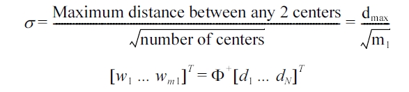
Weights: are computed by means of the pseudo-inverse method.
>
D. Metrics Used to Analyze the Results
We will use three performance metrics to analyze our results.
DR is the ratio between the number of correctly detected attacks and the total number of attacks.
FPR is the ratio between the number of normal connections that are incorrectly misclassified as attacks and the total number of normal connections.
A confusion matrix (CM) is a visualization tool typically used in supervised learning.
This section presents the experimental results detailing the performance of the BPNNIDS and the RBFNNIDS. Both sys-tems are trained on a10% version of the KDD Cup 1999 dataset, and the sample we selected from the 10% version of the KDD Cup 1999 dataset. A Pentium 4 (2.33 GHz) laptop, with 2 GB of memory was used to implement the systems.
>
A. Five Category System using 10% Version of KDD Cup 1999 (FCS 10 KDD)
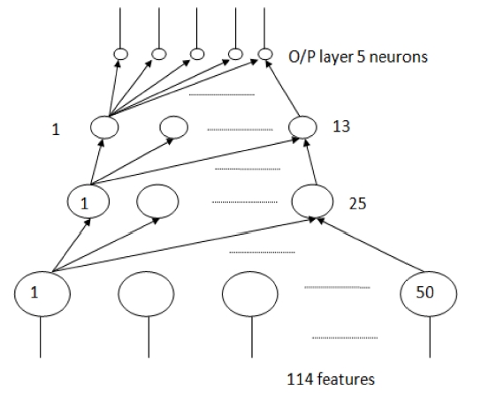
A four layer neural network (Fig. 4) was used. It has three hidden layers. The size of the input, hidden and output layer are 114, 50, 25, 13, and 5 respectively. 114 is the number of features used in the training and 5 is the number of categories.
We first tried a network architecture of two hidden layers, but this did not converge to a solution. Then we increased the hid-den layers to three. The number of neurons in each hidden layer was chosen by trial and error. We started with a size of the first hidden layer at 41 neurons. This is the original number of fea-tures in the dataset. Then, this size was increased until optimum results were obtained. Similarly, the size of 2nd hidden and 3rd hidden layers were chosen. For the parameters, the mean square error (MSE) in the training step is 0.001, transfer sigmoid,learning rule momentum, step size 1.0 and momentum 0.7.
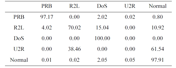
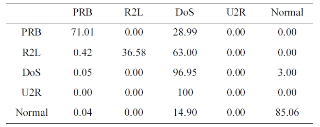
Confusion matrix for BPNNIDS trained by a 10% version of the dataset (five category system)
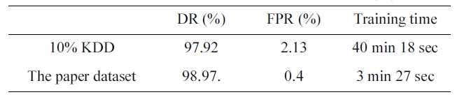
The suggested network architecture was trained using a 10% version of the KDD Cup1999 dataset (Table 1) in 40 minutes and 18 seconds, and then tested using the KDD Corrected testing set (Table 4). The resulting confusion matrix is shown in Table 5.
The training of the neural networks is stopped at 20 epochs, with a minimum MSE of 8.63806E-05
The values at the diagonal of the matrix in Table 5 represent the correct detected records. So, the detection rate can be calcu-lated from Table. 4 and 5 by using the following equation:
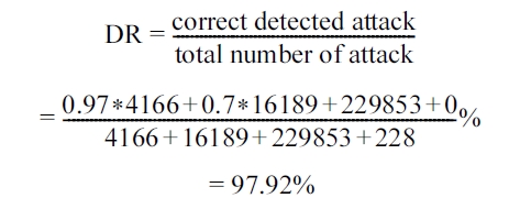
Similarly, the values in the last row of the confusion matrix (Table 5) show the records detected to be normal. The first four values are obviously misclassified as an attack. The false posi-tive rate is calculated as follow:
FPR = 0.01 + 0.02 + 2.05 + 0.05 = 2.13%.
>
B. Five Category System using the Proposed Reduced Dataset (FCS P KDD)
The suggested network architecture is trained using the sam-
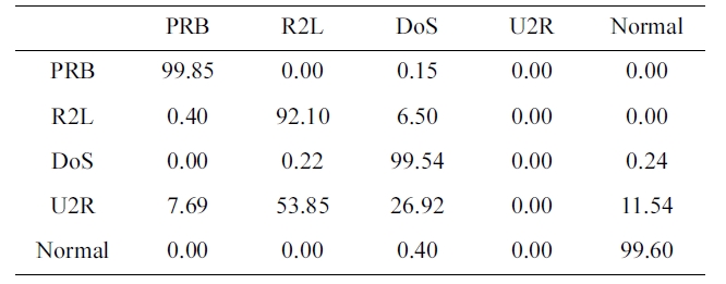
Confusion matrix for BPNNIDS trained by our selected KDD Cup 1999 dataset (five category system)
[Table 7.] Performance under the two datasets (five category system)
Performance under the two datasets (five category system)
ple we selected from a 10% version of the KDD Cup 1999 dataset (Table 2) in 3 minutes and 27 seconds, and tested using the KDD Corrected testing set (Table 4). The resulting confusion matrix is shown in Table 6.
The training of the neural network is stopped at 22 epochs, with minimum MSE of 0.000531693
Similarly, the DR and FPR can be calculated from Table 4 and Table 6 to be:
DR = 98.97%.
FPR = 0.4%.
Comparing Performance under the two sets (FCS)
By comparing the two results, we can conclude that the the dataset we selected has an excellent training time of only 3 min-utes and 27 seconds (Table 7) with a better detection and false positive rate.
>
C. Two Category System using 10% Version of Kdd Cup 1999 (Tcs 10 Kdd)
A four layer neural network was used. It has three hidden layers. The sizes of the input, hidden and output layers are 114, 50, 25, 15, and 2 respectively. 114 is the number of features used in the training and 2 is the number of categories. We chose the number of hidden layers and the number of neurons in each layer in a way similar to that used in the five category system.
For the parameters, the mean square error (MSE) in the train-ing step is 0.001, transfer function is the sigmoid, learning rule is the momentum, the step size is 1.0 and momentum is 0.7.
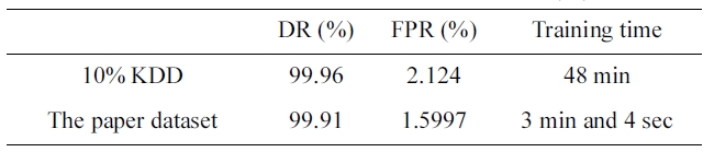
The suggested network architecture is trained using a 10% version of the KDD Cup 1999 dataset (Table 1) in 48 minutes, and tested using the KDD Corrected testing set (Table 4). The resulting confusion matrix is shown in Table 8.
The training of the neural network was stopped at 21 epochs, with minimum MSE of 0.000204713.
[Table 8.] Confusion matrix for BPNNIDS trained by 10% version of dataset (two category system)
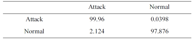
Confusion matrix for BPNNIDS trained by 10% version of dataset (two category system)
Similarly, the DR and FPR can be calculated from Table. 4 and 8 to be:
DR = 99.96%.
FPR = 2.124%.
>
D. Two Category System using the Proposed Reduced Dataset (TCS P KDD)
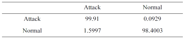
The suggested network architecture is trained using the sam-ple we selected from the 10% version of the KDD Cup 1999 dataset (Table 1) in 3 minutes 4 seconds, and tested using the KDD Corrected testing set (Table 4). The resulting confusion matrix is shown in Table 9.
The training of the neural networks is stopped at 22 epochs, with minimum MSE of 0.000556344.
Similarly, the DR and FPR can be calculated from Table. 4 and 9 to be:
DR = 99.91%
FPR = 1.5997%.
Comparing Performance under the two sets (TCS)
By comparing the two results, we can conclude that the dataset we selected has an excellent training time of only 3 min-utes and 4 seconds (Table 10) with a better detection and false positive rate.
>
E. Five Category System using the Proposed Reduced Dataset and RBF (FCS P KDD)
A four layer neural network is used. It has one RBF layer, two hidden layers and one output layer. The size of the input , RBF, hidden and output layers are 114, 114, 25, 13, and 5
Confusion matrix for BPNNIDS trained by the our selected KDD Cup 1999 dataset (two category system)
[Table 10.] Performance under the two sets (two category system)
Performance under the two sets (two category system)
respectively.
We first tried a network architecture with the number of cen-ters less than the number of features. However, this did not con-verge to a solution. Then, we increased the number of centres to be equal to the number of features. The number of neurons in each hidden layer was chosen by trial and error. We started with the size of the first hidden layer to be 20 neurons. Then, this size was increased until optimum results were obtained. Similarly, the sizes of the two hidden layers were chosen.
For the unsupervised learning parameters, the number of cen-ters is 144, the maximum epochs are 100, termination? weight change is 0.001 and learning rate is varied from 0.01 to 0.001.
For the other parameters, the MSE in the training step is 0.001, transfer function is the sigmoid, learning rule is the momentum, the step size is 1.0 and momentum is 0.7.
The suggested network architecture was trained using the paper sample we selected from the 10% version of the KDD Cup 1999 dataset (Table 2) in 36 minutes 14 seconds, and tested using the KDD Corrected testing set (Table 4), the resulting confusion matrix is shown in Table 11.
By comparing Table. 7 and 11, we can conclude that the pro-posed BPNNIDS has an excellent training time of only 3 min-utes and 4 seconds (Table 10) with a better detection and false positive rate.
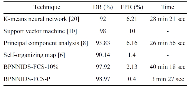
We compare the performance of the paper proposed BPN-NIDS with some of the other neural-network-based approaches, such as K-means NN, SVM, SOM, and PCA. For this purpose, we use the published results in (6, 8, 10, 20). We compare the %DR and %FPR. Table 12 shows the experimental results. Some incomplete items in the published results are represented by ‘_’. The proposed back-propagation neural network intrusion

Confusion matrix for RBF trained by the ourselected KDD Cup 1999 dataset (five category system) without stopping
[Table 12.] Comparison with the previous work

Comparison with the previous work
detection system (BPNNIDS) achieves a higher DR and lower FPR than all the other listed systems in less time.
In this paper, a supervised learning approach to the intrusion detection problem is investigated and demonstrated on the International Knowledge Discovery and Data Mining Tools Competition intrusion detection benchmark (the KDDCUP 99 dataset). To do so this we investigated two architectures; the first engine is a back-propagation neural network intrusion detection system (BPNNIDS) and the second is a RBFNNIDS. The two engines work under two basic data sets; one is limited to 19361 connections (records), which is the set we selected from the 10% version of the KDD Cup 1999 dataset whereas the other contains 494021 connections (records), which is the 10% ver-sion of the KDD Cup 1999 dataset.
The significance of this paper’s iterative reduction algorithm is to reduce the training time from 40 minutes 18 seconds to 3 minutes 27 seconds in the five category system. It also reduces the training time from 48 minutes to 3 minutes and 4 seconds in the two category system.
Our systems include two types of encapsulation. The first one encapsulates the 22 attack types to their four original cate-gories DoS, PRB, R2L, and U2L. The second one encapsulates the 22 attack types to the word attack. Two systems are intro-duced; the first one uses the proposed five category encapsula-tion: DoS, PRB, R2L, U2L, and normal. The second system uses the proposed two category encapsulation: attack and normal.
The proposed iterative reduction algorithm, encoding the symbolic features and the complexity architecture of the pro-posed neural networks had a great effect on ensuring a high DR with a low FPR. The DR was 98.97% and FPR was 0.4% in the five category system that used the back-propagation neural net-works engine with the reduced dataset. The DR was 97.92% and FPR was 2.13% in the five category system that used the back-propagation neural networks engine with the 10% version of the KDD Cup 1999 dataset. The DR was 99.91% and FPR was 1.5997% in the two category system that used the back-propagation neural networks engine with the reduced dataset. The DR was 99.96% and FPR was 2.124% in the two category system that used the back-propagation neural networks engine with the 10% version of the KDD Cup 1999 dataset.
This paper introduced two types of machine learning in a supervised environment. The first one depends on back-propa-gation neural networks and the second one depends on the radial basis function. By comparing the training time, the detec-tion rate and the false positive rate it can be concluded that the engine with the back-propagation neural networks produced better results than the one using the radial basis function.