Over the past few years, keyword search on extensible markup language (XML) data has been a hot research issue, along with the steady increase of XML-based applications [1-12]. As with the importance of effectiveness in keyword search, efficiency is also a key factor in the success of keyword search.

Typically, an XML document is modeled as a nodelabeled tree T. For a given keyword query Q, each result t is a subtree of T containing each keyword of Q at least once, where the root node of t should satisfy a certain semantics, such as smallest lowest common ancestor (SLCA) [4], exclusive lowest common ancestor (ELCA) [2, 3, 9], valuable lowest common ancestor (VLCA) [11] or meaningful lowest common ancestor (MLCA) [5]. Based on the set of qualified root nodes, there are three kinds of subtree results: 1) complete subtree (CSubtree), which is a subtree

rooted at a node v that is excerpted from the original XML tree without pruning any information [2, 4]; 2) path subtree (PSubtree), which is a subtree

that consists of paths from v to all of its descendants, each of which contains at least one input keyword [13]; and 3) matched subtree (MSubtree), which is a subtree

rooted at v satisfying the constraints of monotonicity and consistency [7, 8]. Let S_v' = {k₁,k₂,...k_m'} be the set of distinct keywords contained in the subtree rooted at a node v', S_v'⊆Q. Intuitively, a subtree t_v is an MSubtree if and only if for any descendant node v' of v, there does not exist a sibling node u' of v', such that S_v'⊂S_u' , which we call the constraint of “keywords subsumption”. Obviously, for a given CSubtree

can be got by removing from

all nodes that do not contain any keyword of the given query in their subtrees, and, according to [8],

can be got by removing from

all of the nodes that do not satisfy the constraint of keywords subsumption.

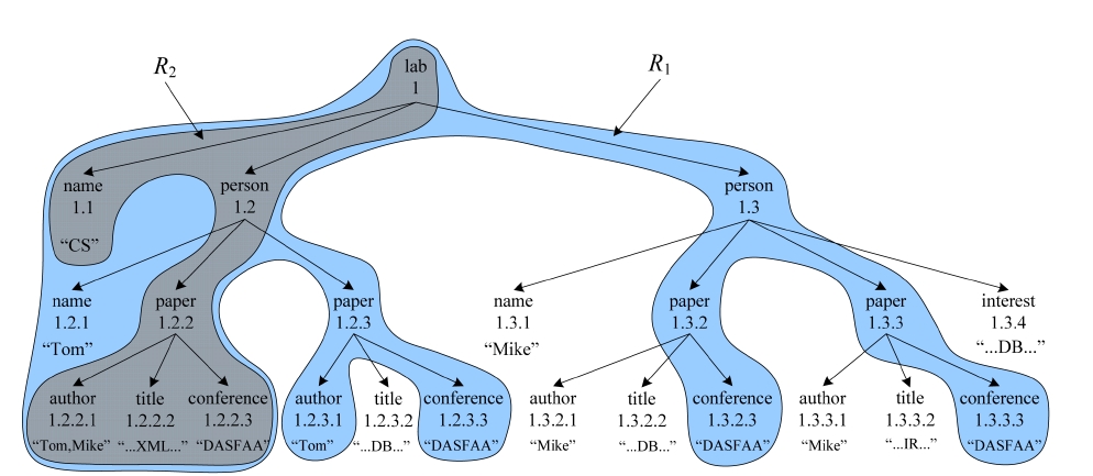
EXAMPLE 1. To find for “CS” laboratory all papers that are written by “Tom” and published in “DASFAA” about “XML” from the XML document D in Fig. 1, we may submit a query Q = {CS, Tom, DASFAA, XML} to complete this task. Obviously, the qualified SLCA node is the root node with Dewey [10] label “1”. Therefore, the CSubtree for Q is D itself, the PSubtree is R₁, while the MSubtree is R2.

From Example 1 we know that a CSubtree, e.g., D, may be incomprehensible for users, since it could be as large as the document itself, while a PSubtree could make users feel frustrated, since it may contain too much irrelevant information, e.g., although each leaf node of R1 directly contains at least one keyword of Q, the three papers with Dewey labels “1.2.3, 1.3.2, 1.3.3” have nothing to do with “XML”. In fact, from Fig. 1 we can easily know that for “CS” laboratory, the paper written by “Tom” and published in “DASFAA” about “XML” is the node with Dewey label “1.2.2”. According to Fig. 1, we know that the keyword sets for nodes 1.1, 1.2, and 1.3 are S_1.1 = {CS}, S_1.2 = {Tom, DASFAA, XML}, and S_1.3 = {DASFAA}, respectively. According to the constraint of keywords subsumption, all nodes in the subtree rooted at node 1.3 should be pruned, since S_1.3⊂S_1.2. Similarly, the keyword sets for node 1.2.1, 1.2.2, and 1.2.3 are S_1.2.1 = {Tom}, S_1.2.2 = {Tom, DASFAA, XML}, and S_1.2.3 = {Tom, DASFAA}, respectively. According to the constraint of keywords subsumption, since S_1.2.1⊂S_1.2.2 and S_1.2.3⊂S_1.2.2, all nodes in the subtrees rooted at node 1.2.1 and 1.2.3 should be removed. After that, we get the MSubtree, i.e., R₂, which contains all necessary information after removing nodes that do not satisfy the constraint of keywords subsumption, and is more self-explanatory and compact.

However, most existing methods [3, 4, 6, 9, 14] that address efficiency focus on computing qualified root nodes, such as SLCA or ELCA nodes, as efficient as possible. In fact, constructing subtree results is not a trivial task. Existing methods [7, 8] need to firstly scan all node

labels to compute qualified SLCA/ELCA results, and then rescan all node labels to construct the initial subtrees. After that, they need to buffer these subtrees in memory, and apply the constraint of keywords subsumption on each node of these subtrees, to prune nodes with keyword sets subsumed by that of their sibling nodes, which is inefficient in time and space.

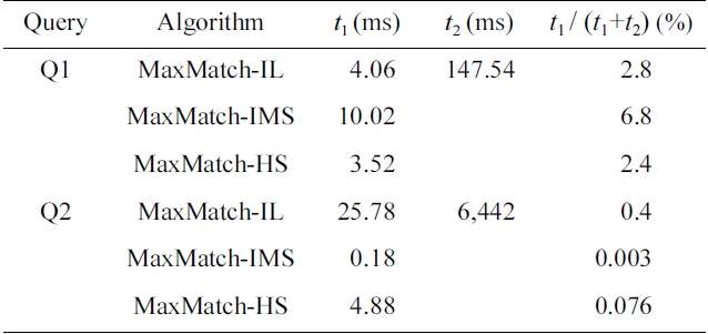
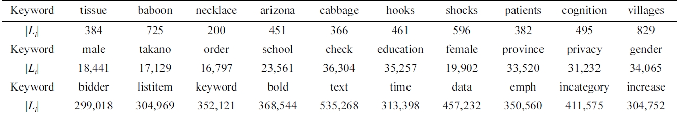
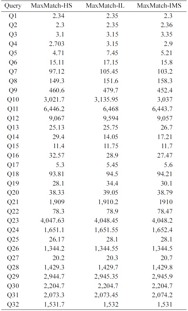
EXAMPLE 2. Take the MaxMatch algorithm [8] for example. It firstly gets the set of SLCA nodes based on either indexed lookup (IL) [4], incremental multiway SLCA (IMS) [6] or hash search (HS) [12] algorithm, then computes all matched subtree results. We ran the Max- Match algorithm for query Q1 = {school, gender, education, takano, province} and Q2 = {incategory, text, bidder, data} on the XMark (http://monetdb.cwi.nl/xml) dataset of 582 MB. We found that no matter which one of IL, IMS, and HS is adopted, the time of SLCA computation is less than 7% and 1% of the overall running time for Q1 and Q2, respectively, as shown in Table 1.

From Example 2 we know that, given a set of SLCA nodes, the operation of computing matched subtree results will dominate the overall performance of the MaxMatch algorithm, thus should deserve being paid more attention. As illustrated by [7], an MSubtree could still contain redundant information; e.g., the four conference nodes, i.e., 1.2.2.3, 1.2.3.3, 1.3.2.3, and 1.3.3.3, of D in Fig. 1 are the same as each other according to their content, and for keyword query {CS, conference}, returning only one of them is enough. However, the MSubtree result contains all of these conference nodes, because all of them satisfy the constraint of keywords subsumption.

In this paper, we focus on constructing tightest matched subtree (TMSubtree) results according to SLCA semantics. Intuitively, a TMSubtree is an MSubtree after removing redundant information, and it can be generated from the corresponding PSubtree by removing all nodes that do not satisfy the constraint of keywords subsumption, and just keeping one node for a set of sibling nodes that

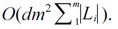
have the same keyword set. Assume that d is the depth of a given TMSubtree, m is the number of keywords of the given query Q. We proved that if d ≤ m, then a TMSubtree has at most 2m! nodes; otherwise, the number of nodes of a TMSubtree is bounded by (d ? m 2) m!. Based on this theoretical result, we propose a pipelined algorithm to compute TMSubtrees without rescanning all node labels. Our algorithm sequentially processes all node labels in document order, and immediately outputs each TMSubtree once it is found. Compared with the MaxMatch algorithm [8], our method reduces the space complexity from

to O(d · max{2m!, (d - m + 2)· m!}), where L_i is the inverted Dewey label list of keyword k_i.

The rest of the paper is organized as follows. In Section II, we introduce background knowledge, and discuss the related work. In Section III, we give an in-depth analysis of the MaxMatch algorithm [8], then define the tightest matched subtree (TMSubtree) and discuss its properties, and finally, present our algorithm on computing all TMSubtree results. In Section IV, we present the experimental results, and in Section V, we conclude our paper.

† An earlier version of this paper has been published at DASFAA 2012.

We model an XML document as a node labeled ordered tree, where nodes represent elements or attributes, while edges represent direct nesting relationships between nodes in the tree. Fig. 1 is a sample XML document. We say a node v directly contains a keyword k, if k appears in the node name or attribute name, or k appears in the text value of v.

A Dewey label of node v is a concatenation of its parent's label and its local order. The last component is the local order of v among its siblings, whereas the sequence of components before the last one is called the parent label. In Fig. 1, the Dewey label of each node is marked as the sequence of components separated by “.”. For a Dewey label A: a₁.a₂...a_n, we denote the number of components of A as |A|, and the i^th component as A[i]. As each Dewey label [10] consists of a sequence of components representing the path from the document root to the node it represents, the Dewey labeling scheme is a natural choice of state-of-the-art algorithms [2, 4, 6, 15, 16] for keyword query processing on XML data. The positional relationships between two nodes include document order (？_d), equivalence (=), ancestor-descendant (AD, ?_a), parent- child (PC,?_p), ancestor-or-self (?_a) and Sibling relationship. u？_d v means that u is located before v in document order, u ?_a v means that u is an ancestor node of v, and u?_p v denotes that u is the parent node of v. If u and v represent the same node, we have u = v, and both u?_d v and u?_a v hold. In the following discussion, we do not differentiate between a node and its label, if without ambiguity.

For a given query Q = {k₁, k₂, …, k_m} and an XML document D, we use L_i to denote the inverted Dewey label list of k_i, of which all labels are sorted in document order. Let LCA(v₁, v₂,...., v_m) be the lowest common ancestor (LCA) of nodes v₁, v₂,..., v_m, the LCAs of Q on D are defined as LCA(Q) = {v|v = LCA(v₁, v₂,…, v_m), v_i∈L_i(1≤i≤m)}; e.g., the LCAs of Q ={XML, Tom} on D in Fig. 1 are nodes 1.2 and 1.2.2.

In the past few years, researchers have proposed many LCA-based semantics [1, 2, 4, 5, 11], among which SLCA [4, 6] is one of the most widely adopted semantics. Compared with LCA, SLCA defines a subset of LCA(Q), of which no LCA in the subset is the ancestor of any other LCA, which can be formally defined as SLCASet = SLCA(Q) = {v|v∈LCA(Q) and ?v'∈LCA(Q), such that v ?_a v'}. In Fig. 1, although 1.2 and 1.2.2 are LCAs of Q = {XML, Tom}, only 1.2.2 is an SLCA node for Q, because 1.2 is an ancestor of 1.2.2.

Based on the set of matched SLCA nodes, there are three kinds of subtree results: 1) CSubtree [2, 4]; 2) PSubtree [13]; and 3) MSubtree, which is a subtree rooted at v satisfying the constraints of monotonicity and consistency [7, 8], which can be further interpreted by the changing of data and query, respectively. Data monotonicity means that if we add a new node to the data, the number of query results should be (non-strictly) monotonically increasing. Query monotonicity means that if we add a keyword to the query, then the number of query results should be (non-strictly) monotonically decreasing. Data consistency means that after a data insertion, each additional subtree that becomes (part of) a query result should contain the newly inserted node. Query consistency means that if we add a new keyword to the query, then each additional subtree that becomes (part of) a query result should contain at least one match to this keyword. [8] has proved that if all nodes of a subtree t_v satisfy the constraint of “keywords subsumption”, then t_v must satisfy the constraints of monotonicity and consistency, that is, t_v is an MSubtree. According to Example 1, we know that compared with CSubtrees and PSubtrees, MSubtrees contain all necessary information after removing nodes that do not satisfy the constraint of keywords subsumption, and are more self-explanatory and compact.

To construct MSubtrees, the existing method [8] needs to firstly scan all node labels to compute qualified SLCA nodes, then rescan all node labels to construct the initial subtrees. After that, they need to buffer these subtrees in memory and apply the constraint of keywords subsumption on each node of these subtrees to prune nodes with keyword sets subsumed by that of their sibling nodes, which is inefficient in time and space.

Considering that an MSubtree may still contain redundant information (discussed in Section I), in this paper, we focus on efficiently constructing TMSubtree results based on SLCA semantics. Intuitively, a TMSubtree is an MSubtree, after removing redundant information. Constructing TMSubtree results based on ELCA semantics [7] is similar, and therefore omitted for reasons of limited space.

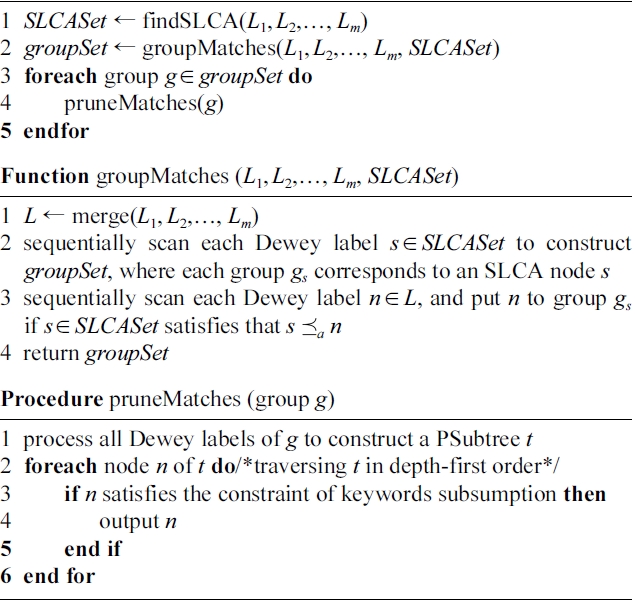
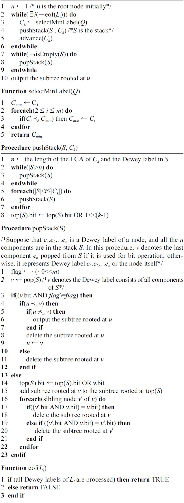
The MaxMatch algorithm [8] returns MSubtree results that are rooted at SLCA nodes, and satisfy the constraint of “keywords subsumption”. For a given query Q = { k₁,…,k_m} and an XML document D, supposing that L₁(L_m) is the Dewey label list of occurrence of the least (most) frequent keyword of Q, d is the depth of D. As shown in Algorithm 1, the MaxMatch algorithm works in three steps to produce all MSubtree results.

Step 1 (line 1): MaxMatch finds from the m inverted Dewey label lists the set of SLCA nodes, i.e., SLCASet, by calling the IL algorithm [4]. The cost of this step is O(md|L₁| log |L_m|). In this step, all Dewey labels are processed once. Note that any algorithm for SLCA computation can be used in this step.

Step 2 (line 2): MaxMatch calls function groupMatches to construct the set of groups, i.e., groupSet. As shown in

groupMatches, it needs to firstly merge the m lists into a single list with cost

then sequentially rescan all labels and insert each one to a certain group (if possible), with cost

in this step, all Dewey labels are processed twice to construct the set of groups.

Step 3 (lines 3-5): For each group g, MaxMatch firstly constructs the PSubtree, then traverses it to prune redundant information. The overall cost of Step 3 is O(min{|D|,

}·2^m), where 2^m is the cost of checking whether the set of distinct keywords of node v is subsumed by that of its sibling nodes; if not, then v is a node that satisfies the constraint of keywords subsumption.

Therefore, the time complexity of Algorithm 1 is O(max {min{|D|,

}·2^m, md|L₁|log|L_m|}). Moreover, as the MaxMatch algorithm needs to buffer all groups in memory before step 3, its space complexity is

DEFINITION 1. (TMSubtree) For an XML tree D and a keyword query Q, let S_v⊆Q be the set of distinct keywords that appear in the subtree rooted at v, S_v≠Φ. A subtree t is a TMSubtree iff t’s root node is an SLCA node, and each node v of t satisfies that for each sibling node v' of v, S_v?S_v', and for each set of sibling nodes {v₁,v₂, …, v_n} satisfying S_v1 = S_v2 =…= S_vn, only one of them is kept for presentation.

Intuitively, a TMSubtree is an MSubtree with redundant information being removed. It can be generated from the corresponding PSubtree by removing all nodes that do not satisfy the constraint of keywords subsumption, and just keeping one node for a set of sibling nodes that have the same keyword set.

DEFINITION 2. (Maximum TMSubtree) Let t be a TMSubtree of Q, v a node of t, S_v⊆Q the set of distinct keywords that appear in the subtree rooted at v, v.level the level value of v in t. We say t is a maximum TMSubtree if it satisfies the following conditions:

1) v has|S_v| child nodes v₁, v₂,… , v_|Sv|,

2) if |S_v|≥2？v.level < d, then for any two child nodes v_i, v_j(1≤i ≠j≤|S_v|), |S_vi| = |S_vj| =|S_v| ？ 1？|S_vi？S_vj| = |S_v| ? 2,

3) if |S_v| = 1？v.level < d, then v has one child node v₁ and S_v = S_v1.

LEMMA 1. Given a maximum TMSubtree t, t is not a TMSubtree anymore, after inserting any keyword node into t without increasing t's depth.

Proof. Suppose that t is not a maximum matched subtree result, then there must exist a non-leaf node v of t, such that we can insert a node v_c into t as a child node of v; v_c satisfies that S_vc⊆S_v . Obviously, there are four kinds of relationships between S_vc and S_v:

1) |S_vc| = |S_v| = 1. In this case, v has one child node that contains the same keyword as v. Obviously, v_c cannot be inserted into t, according to Definition 1.

2) S_vc = S_v ？|S_v| ≥ 2. Since v has |S_v| child nodes and each one contains |S_v|?1 keywords, for each child node v_i (1≤i≤|S_v|) of v, we have S_vi⊂S_v = S_vc. According to Definition 1, all existing child nodes of v should be removed if v_c is inserted into t, thus v_c cannot be inserted into t as a child node of v, in such a case.

3) |S_vc| = |S_v| ?1？|S_v| ≥ 2. According to condition 2, all existing child nodes of v contain all possible combinations of keywords in S_v, thus there must exist a child node v_ci of v, such that S_vc = S_vci, which contradicts Definition 1, thus v_c cannot be inserted into t in this case.

4) if |S_vc| <|S_v| ？ 1？|S_v| ≥ 2. According to condition 2, all existing child nodes of v contain all possible combinations of keywords in S_v, thus there must be a child node v_ci of v, such that S_vc⊂S_vci, which also contradicts Definition 1, thus v_c cannot be inserted into t in such a case.

In summary, if t is a maximum TMSubtree result, no other keyword node can be inserted into t, such that t is still a TMSubtree, without increasing t’s depth.

THEOREM 1. Given a keyword query Q = {k₁, k₂,..., k_m} and one of its TMSubtree t of depth d, if d ≤ m, then t has at most 2m! nodes; otherwise, the number of nodes of t is bounded by (d ? m 2) m!.

Proof. Assume that t is a maximum TMSubtree, obviously, the number of nodes at 1^st level of t is 1 =

For the 2^nd level, since S_t.root = Q, t.root has |S_t.root| =

child nodes, of which each one contains |S_t.root| ? 1 distinct keywords.

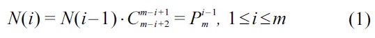
Thus we have Formula 1 to compute the number of nodes at the i^th level.

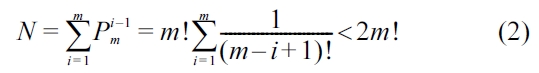
If d ≤ m, the total number of nodes in t is

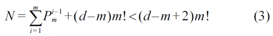
If d > m, each node at the m^th level of t contains only one keyword, and all levels greater than m contain the same number of nodes as that of the m^th level. According to Formula 1, we know that N(m) = m!, thus the total number of nodes in t is

Therefore if d ≤ m, a TMSubtree t has at most 2m! nodes, otherwise, the number of nodes of t is bounded by (d ? m 2)· m!.

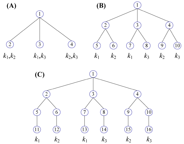
EXAMPLE 3. Given a keyword query Q = {k₁, k₂, k₃}, Fig. 2 shows three subtree results; according to Definition 1, they are all TMSubtrees. Obviously, by fixing their depths, no other node with any kind of combination of k₁ to k₃ can be inserted into these TMSubtree results, according to Lemma 1, that is, they are all maximum TMSubtrees. The TMSubtree in Fig. 2a has 4 nodes. Since its depth is 2 and is less than the number of keywords, i.e., 3, it satisfies Theorem 1, since 4 < 2 × 3! = 12. The TMSubtree in Fig. 2b is another maximum TMSubtree with 10 nodes, and also satisfies Theorem 1, since 10 < 2 × 3! = 12. Fig. 2c is also a maximum TMSubtree with 16 nodes. Since the depth of the TMSubtree is 4 and is greater than the number of keywords of Q, it still satisfies Theorem 1, since 16 < (4 ? 3 2) × 3! = 18.

Compared with the MaxMatch algorithm that produces all subtree results in three steps, the basic idea of our method is directly constructing all subtree results in the procedure of processing all Dewey labels. The benefits of our method lie in two aspects: 1) the buffered data in memory is largely reduced; 2) each Dewey label is visited only once. The first benefit comes from Theorem 1, which guarantees that our method does not need to buffer huge volumes of data in memory as [8] does; the second benefit is based on our algorithm.

In our algorithm, for a given keyword query Q = {k₁, k₂,..., k_m}, each keyword k_i corresponds to a list L_i of Dewey labels sorted in document order, and L_i is associated with a cursor C_i pointing to some Dewey label of L_i. C_i can move to the Dewey label (if any) next to it by using advance(C_i). Initially, each cursor C_i points to the first Dewey label of L_i.

As shown in Algorithm 2, our method sequentially scans all Dewey labels in document order. The main procedure is very simple: for all nodes that have not been visited yet, in each iteration, it firstly chooses the currently minimum Dewey label, by calling the selectMin- Label function (line 3), then processes it, by calling the pushStack procedure (line 4), and finally, it moves C_k forwardly to the next element in L_k (line 5). After all Dewey labels are processed, our algorithm pops all in-stack elements (line 7-9), then outputs the last TMSubtree result, to terminate the processing (line 10).

During the processing, our algorithm uses a stack S to temporarily maintain all components of a Dewey label, where each stack element e denotes a component of a Dewey label, which corresponds to a node in the XML tree. e is associated with two variables: the first one is a binary bitstring indicating which keyword is contained in the subtree rooted at e; the second is a set of pointers pointing to its child nodes, which is used to maintain intermediate subtrees.

The innovation of our method lies in that our method immediately outputs each TMSubtree result t_v when finding v is a qualified SLCA node, which makes it more efficient in time and space. Specifically, in each iteration (line 2 to 6 of Algorithm 2), our method selects the currently minimum Dewey label C_k in line 3, then pushes all components of C_k into S in line 4. The pushStack procedure firstly pops from S all stack elements that are not the common prefix of C_k and the label represented by the current stack elements, then pushes all C_k's components that are not in the stack into S. To pop out an element from S, the pushStack procedure will call popStack procedure to complete this task. The popStack procedure is a little more tricky. It firstly checks whether the popped element v is an LCA node. If v is not an LCA node, popStack firstly transfers the value of v's bitstring to its parent node in S (line 14), then inserts subtree t_v into t_top(S) in line 15. In lines 16 to 22, popStack will delete all possible redundant subtrees, by checking the subsumption relationship between the keyword set of v and that of its sibling nodes. If v is an LCA node (line 3) and located after the previous LCA node u in document order (line 4), it means that u is an SLCA node if it is not an ancestor of v (line 5), then popStack directly outputs the TMSubtree result rooted at u in line 6. The subtree rooted at u is then deleted (line 8), and u points to v in line 9. If v is an LCA node but located

before u, it means that v is not an SLCA node, thus we directly delete the subtree rooted at v (line 11).

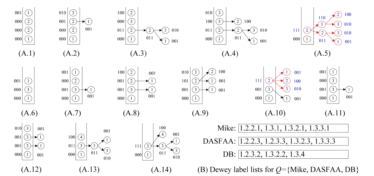
Example 4. Consider the XML document D in Fig. 1 and query Q = {Mike, DASFAA, DB}. The inverted Dewey label lists for keywords of Q are shown in Fig. 3b. The status of processing these labels is shown in Fig. 3a1-a14. In this example, we use “001” (“010” or “100”) to indicate that “Mike” (“DASFAA” or “DB”) is contained in a subtree rooted at some node. After 1.2.2.1 is pushed into stack, the status is shown in Fig. 3a1, where the bitstring of the top element of S is “001”, indicating that node 1.2.2.1 contains “Mike”. The second pushed label is 1.2.2.3, and the status is shown in Fig. 3a2. Note that after an element is popped out from the stack, its bitstring is transferred to its parent in the stack. The next two labels are processed similarly. Before 1.3.1 is pushed into the stack, we can see from Fig. 3a5 that the bitstring of the top element in S is “111”, which means that node 1.2 contains all keywords. After 1.3.1 is pushed into stack, the subtree rooted at 1.2 is temporarily buffered in memory. As shown in Fig. 3a10, before 1.3.3.1 is pushed into stack, the last component of 1.3.2 will be popped out from the stack. Since the bitstring of the current top element in S is “111” (Fig. 3a10), we know that 1.3.2 is an LCA node. According to line 5 of popStack procedure, we know that the previous LCA, i.e., 1.2, is an SLCA node, thus we output the matched subtree result rooted at 1.2. After that, the subtree rooted at 1.3.2 will be temporarily buffered in memory. When the last component of 1.3 is popped out from S (Fig. 3a14), according to line 3 of popStack procedure, we know that 1.3 is an LCA node. According to line 4 of popStack procedure, we know that the previous LCA node, i.e., 1.3.2, is located after 1.3 in document order, thus we know that 1.3 is not an SLCA node immediately, and delete the subtree rooted

at 1.3 in line 11 of popStack procedure. Finally, we output the TMSubtree rooted at 1.3.2 in line 10 of Algorithm 2. Therefore for Q, the two TMSubtree results are rooted at 1.2 and 1.3.2, respectively.

As shown in Algorithm 2, for a given keyword query Q = {k₁, k₂,..., k_m} and an XML document D of depth d, our method just needs to sequentially scan all labels in the m inverted label lists once, therefore the overall I/O cost of Algorithm 2 is

Now we analyze the time complexity of our algorithm. Since our algorithm needs to process all components of each involved Dewey label of the given keyword query Q = {k₁, k₂, …, k_m}, the total number of components processed in our method is bounded by

, and the cost of processing these components is dm

During processing, each one of the

components will be inserted into a subtree and deleted from the same subtree just once, and the cost of both inserting and deleting a component is O(1). When inserting a subtree into another subtree, the operation of checking the subsumption relationship between the two keyword sets of two sibling nodes will be executed at most m times, according to Definition 2. Therefore, the overall time complexity is

Since our method is executed in a pipelined way, at any time it just needs to maintain at most d subtrees, where each one is not greater than a maximum TMSubtree. According to Theorem 1, each matched subtree result contains at most max{2m!,(d ? m 2)m!} nodes. Therefore, the space complexity of our method is O(d·max{2m!, (d ? m 2)m!}). Since d and m are very small in practice, the size of these subtrees buffered in memory is very small.

Note that to output the name of nodes in a TMSubtree result, existing methods may either store all path infor-mation in advance, by suffering from huge storage space [1], or use the extended Dewey labels [17], by affording additional cost on computing the name of each node, according to predefined rules. In contrast, our method

maintains another hash mapping between each path ID and the path information; the total number of index entries is the number of nodes in the dataguide index [18] of the XML tree, which is very small in practice. To derive for each node its name on a path, we maintain in each Dewey label a path ID after the last component, thus we can get the name of each node on a path in constant time.

Our experiments were implemented on a PC with Pentium(R) Dual-Core E7500 2.93 GHz CPU, 2 GB memory, 500 GB IDE hard disk, and Windows XP professional as the operating system.

The algorithms used for comparison include the Max- Match algorithm (the MaxMatch algorithm is used to output TMSubtrees in our experiment) [8] and our merge- Matching algorithm. MaxMatch was implemented based on IL [4], IMS [6] and HS [12] to test the impacts of different SLCA computation algorithms on the overall performance, and is denoted as MaxMatch-IL, MaxMatch- IMS and MaxMatch-HS, respectively. All these algorithms and our mergeMatching algorithm were implemented using Microsoft VC+ . All results are the average time, by executing each algorithm 100 times on hot cache.

We use XMark dataset for our experiments, because it possesses a complex schema, which can test the features of different algorithms in a more comprehensive way. The size of the dataset is 582 MB; it contains 8.35 million nodes, and the maximum depth and average depth of the XML tree are 12 and 5.5, respectively.

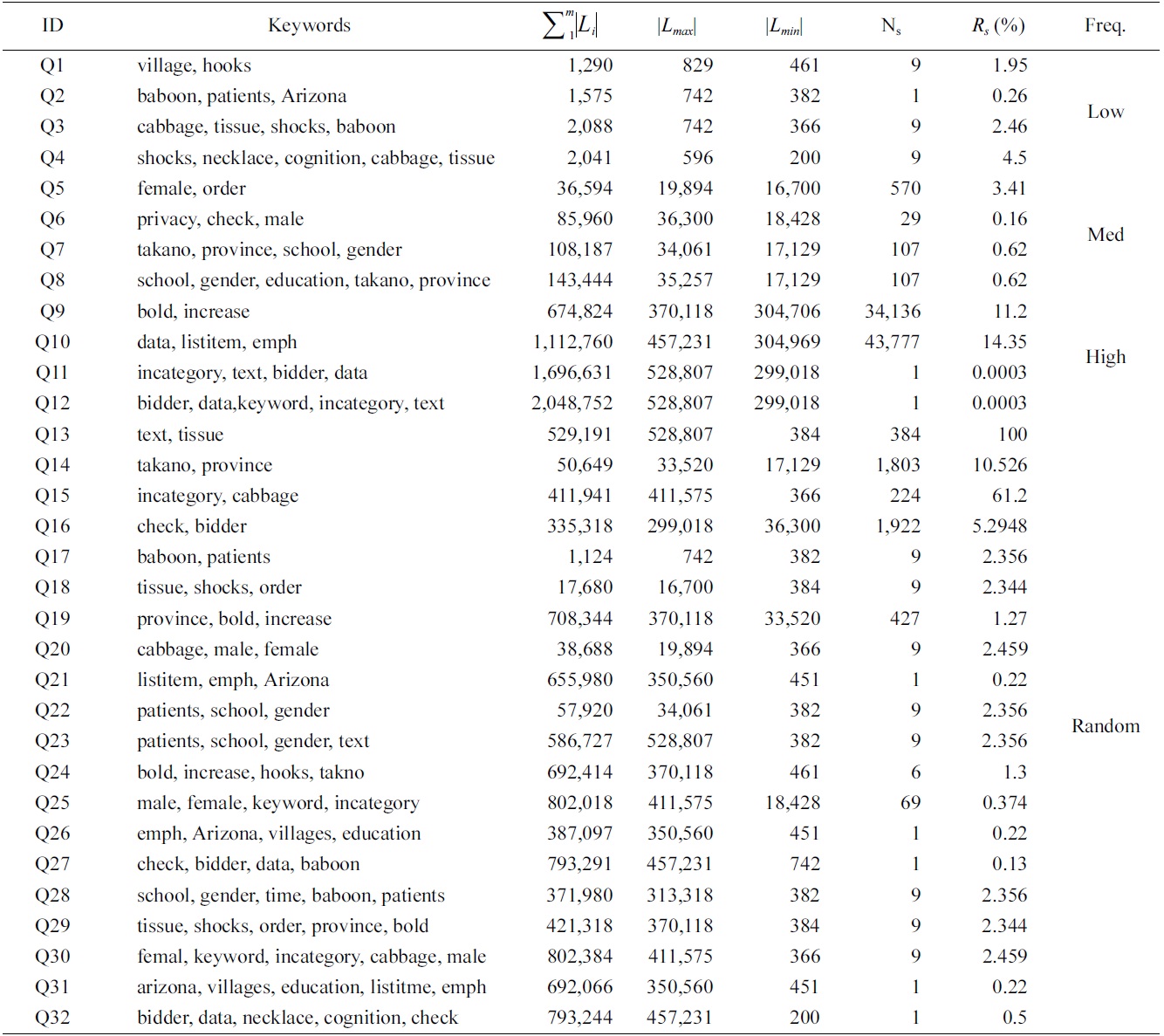
We have selected 30 keywords, which are classified into three categories, according to the length of their inverted Dewey label lists (the |L_i| line in Table 2): 1) low frequency (100-1,000); 2) median frequency (10,000- 40,000); and 3) high frequency (300,000-600,000).

Based on these keywords, we generated four groups of queries, as shown in Table 3: 1) four queries (Q1 to Q4) with 2, 3, 4, 5 keywords of low frequency; 2) four queries (Q5 to Q8) of median frequency; 3) four queries (Q9 to Q12) of high frequency; and 4) 20 queries (Q13 to Q32) with keywords of random frequency.

The metrics used for evaluating these algorithms include: 1) the number of buffered nodes, which is used to compare the space cost of these algorithms, 2) running time on SLCA and subtree result computation, and 3) scalability.

For a given query, we define the result selectivity as the size of the results over the size of the shortest inverted list. The second to last column of Table 3 is the result selectivity of each query.

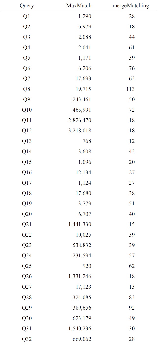
1) Comparison of the Number of Buffered Nodes

To make comparison of space cost for different algorithms, we have collected the statistics of the number of buffered nodes for the MaxMatch and mergeMatching algorithms. Table 4 shows a comparison of the number of buffered nodes for each query, from which we know that the number of buffered nodes for mergeMatching is

much less than that of MaxMatch. The reason lies in that MaxMatch needs to firstly construct all path subtrees and buffer them in memory, while mergeMatching just needs to buffer at most d TMSubtrees in memory, where d is the depth of the given XML tree.

2) Comparison of SLCA Computation:

To get all matched subtree results, the first critical step is computing all qualified SLCA nodes. Fig. 4 shows the comparison of different algorithms on SLCA computation.

From Fig. 4 we have the following observations: 1) mergeMatching is beaten by HS, IL and IMS for almost all queries. This is because mergeMatching sequentially processes all involved Dewey labels. Its performance is dominated by the number of involved Dewey labels, while IL and IMS are more flexible in utilizing the positional relationship to prune useless keyword nodes; HS only sequentially processes each Dewey label of the shortest inverted Dewey label list L₁, and its performance is dominated by the length of L₁. 2) HS is more efficient than IL and IMS when there exists huge difference between the set of involved Dewey label lists, such as Q13, Q15, Q17 to Q32, while it is beaten by IMS when the result selectivity is low, such as Q11 and Q12. This is because HS needs to process all Dewey labels of the shortest list, while IMS can wisely skip many useless nodes. 3) IL can beat IMS for some queries, while it can also be beaten by IMS for other queries, especially when the result selectivity is low, such as Q6, Q11 and Q12. This is because the IL algorithm computes the SLCA results by processing two lists each time from the shortest to the longest, while the IMS algorithm computes each potential SLCA by taking one node from each Dewey label list in each iteration. IMS could be the best choice when all nodes of the set of lists are not uniformly distributed; IL could perform best when all nodes are uniformly distributed, and there exists huge difference in lengths of the set of lists.

3) Impacts of the SLCA Computation on the Overall Performance

To further investigate the impacts of SLCA computation on the overall performance, we implemented the MaxMatch algorithm based on IL, IMS, and HS, which are denoted as MaxMatch-IL, MaxMatch-IMS, and Max- Match-HS, respectively. As shown in Table 5, the three algorithms always consume similar running time, and in most cases, MaxMatch-HS is a little better than the other two algorithms. The reason lies in that they all share the same procedure in constructing matched subtree results, which usually needs much more time than computing SLCA nodes. Therefore, even though HS performs better than IL and IMS in most cases, their overall performance is similar to each other.

Further, from Fig. 4 and Table 5 we know that no matter how efficient HS, IL, and IMS are, and no matter how much HS performs better than IL and IMS, or vice versa, their performance benefits on SLCA computation do not

exist anymore, if compared with the time on constructing matched subtree results based on the MaxMatch algorithm.

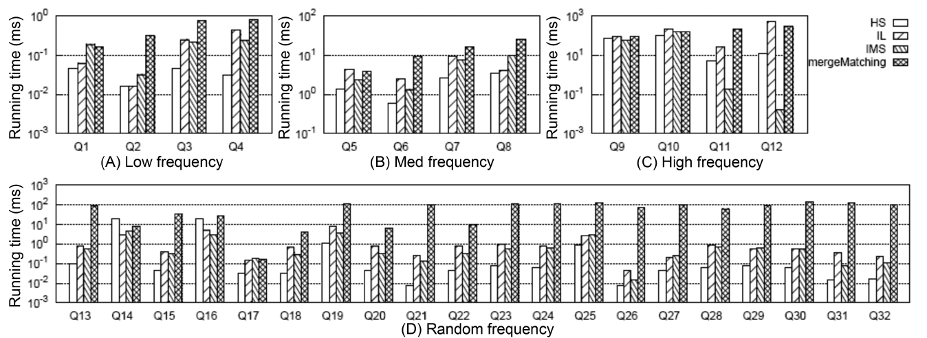
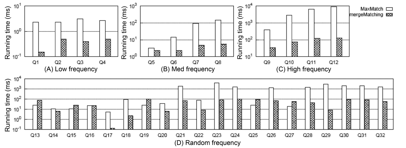
4) Comparison of Constructing Subtree Results

Fig. 5 shows the comparison between MaxMatch and mergeMatching on constructing all matched subtree results, from which we know that although mergeMatching is not as efficient as HS, IL, and IMS on SLCA computation, it is much more efficient than MaxMatch on constructing matched subtree results, such as Q1 to Q12, Q17, Q18, Q20 to Q24, Q26, and Q28 to Q32, and the time saved in the second phase is much more than that wasted in the first phase. The reason lies in that merge- Matching processes each Dewey label only once, while MaxMatch needs to firstly scan all Dewey labels once to compute SLCA results, then scan all Dewey labels once more to construct a set of initial groups according to different SLCA nodes. After that, it constructs all path subtree results by processing these Dewey labels again.

At last, it needs to traverse all nodes to prune useless nodes.

5) Comparison of the Overall Performance

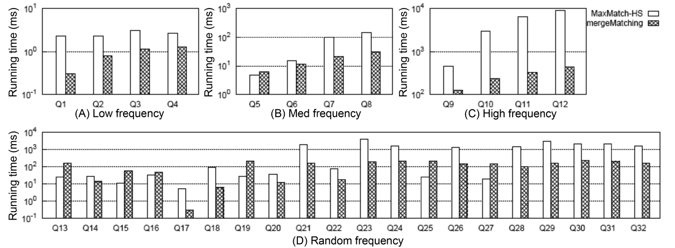
Fig. 6 shows the comparison of the overall running time between MaxMatch-HS and mergeMatching, from which we know that in most cases, mergeMatching performs much better than MaxMatch-HS. The reason lies in that compared with MaxMatch, mergeMatching does not need to rescan all involved Dewey labels, and does not need to delay prune useless nodes after constructing all path subtree results.

On the contrary, it prunes useless nodes when constructing each matched subtree result, and thus can quickly reduce the number of testing operations of the keywords consumption relationship between sibling nodes.

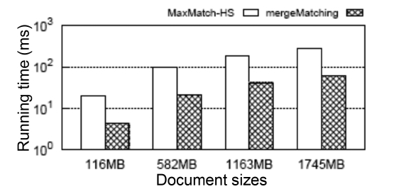
Besides, we show in Fig. 7 the scalability when executing Q7 on XMark datasets with different sizes (from 116 MB to 1745 MB [15x]). The query time of the MaxMatch- HS and our mergeMatching algorithms grow sublinearly with the increase of the data size. Also, mergeMatching consistently saves about 78% time when compared with MaxMatch-HS. For other queries, we have similar results, which are omitted due to limitations of space.

Considering that TMSubtree is more self-explanatory and compact than CSubtree and PSubtree, but existing methods on subtree result computation need to rescan all Dewey labels, we focus in this paper on efficient construction of TMSubtree results for keyword queries on XML data based on SLCA semantics. We firstly proved the upper bound for the size of a given TMSubtree, that is, it has at most 2m! nodes if d ≤ m; otherwise, its size is bounded by (d-m 2)· m!, where d is the depth of a given TMSubtree, and m is the number of keywords of the given query Q. Then we proposed a pipelined algorithm to accelerate the computation of TMSubtree results, which only needs to sequentially scan all Dewey labels once without buffering huge volumes of intermediate results. Because the space complexity of our method is O(d · max {2m!, (d-m 2)· m!}), and in practice, d and m are very small, the size of the buffered subtrees is very small. The experimental results in Section IV verify the benefits of our algorithm in aiding keyword search over XML data.