Web services are web-enabled, platform-independent, loosely coupled, self-contained, and programmable applications that can be described, published, discovered, coordinated, and configured using extensible markup language (XML) artifacts (open standards), for the purpose of developing distributed interoperable applications. Due to the wide application of service-oriented architecture (SOA), large quantities of Web services have been deployed over the Internet or the Web for service users. As the requirements from service users become more and more complicated, an atomic service often can not handle a request by itself, due to its own limited capability. This calls for composite services to combine existing distributed atomic services, thus enabling the performance of more complicated functionalities. The selection of component services (atomic services) for a composite service is a vital yet arduous process. This is because on one hand, the number of alternative Web services which provide the same functionality but differ in quality parameters is growing quickly; while on the other hand, inappropriate selection of component services can result in the degradation of a composite service in terms of the quality of service (QoS). For example, for a composite service that contains a parallel structure, the response time of the composite service is dependent on the component service having the maximum response time (denoted as cmmax) rather than the other ones within the parallel module. Therefore the service selection in the parallel module is designed to make sure the response time of the cmmax is as small as possible. If we take into account the dynamics of Web service environments, the service selection will become even more complicated. This is because the “current-best” candidate service for a component service may not be the best at a later time. In dynamic Web service environments, the performance of the Internet is unpredictable; the reliability and effectiveness of remote Web services are also unclear. Therefore, it cannot be guaranteed that the QoS attributes of Web services will not fluctuate with the dynamic Web service environments. Specifically, we will list three reasons for this dynamic fluctuation: 1) Overwhelming service requests: an overload of the service server will give rise to a fluctuation of the overall performance of a provided service, and usually this fluctuation turns into QoS degradation (e.g., a longer response time); 2) Network performance: some QoS attributes (e.g., response times) may vary or are subject to the quality of the network (e.g., long latency, network disconnection, etc.); 3) Intentional behaviors: sometimes service providers intentionally do not deliver their claimed QoS, in order to, for example, reduce costs or for other purposes.
In this paper, we focus on the two former reasons that may lead to QoS fluctuation. One serious consequence of the aforementioned QoS degradation is the increase in response time. As an important metric of QoS criteria, the growth of response time, meaning service users need to wait for a longer time than they expect, may even result in an unacceptable completion time. Thus in turn results in considerable losses to service users (e.g., lost business revenue, time, or penalties incurred by missing contractual deadlines).
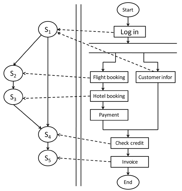
We observe that in the context of dynamic service environments, few works have taken concurrency into consideration when a composite service is planned. By concurrency we mean here that multiple requests to a composite service arrive simultaneously. We demonstrate our work with a classic example in the Web services world, i.e., TripPlanning process (composite service) as shown in Fig. 1. This TripPlanning process can be composed using several tasks, such as flight booking, hotel booking, payment, and so on. Each task can be performed by a concrete service, as denoted by the dashed directed lines which connect the tasks and corresponding services. When a user request arrives at the TripPlanning service, the composite service takes charge of deciding how to offer a satisfactory composition solution for this request. Specifically, this composite service should designate the most desirable concrete service to perform the functionality of each task, thereby accomplishing the user’s request. According to the traditional service selection scheme, the composition solution, which is based on a utility function and aggregates all the values from all the dimensions with respect to QoS into a single value, decides the most desirable candidate services for a given request.
For simplicity sake, we will only consider two services
in this example, namely; flight service (S2) and hotel service (S3). Assume that there are three candidate services (s21, s22, and s23) which can perform the functionality of flight service and two candidate services (s31 and s32) which can do the same for hotel service. Let us further assume that the best composition scheme of the TripPlanning process for the flight service and hotel service, respectively, is selected so that when this composite service receives a request, it will employ s21 and s31 to execute the functionalities of flight service and hotel service. So far in the industry there have been a lot of real-time systems such as real-time ticket ordering systems, stock trading systems, navigational driving guides, etc., which have been characterized by timeliness and lots of concurrent requests. In this context, the arrival frequency of requests is sometimes much higher than the update frequency of the QoS. Suppose for our example that there are 1,000 requests to the TripPlanning process arriving concurrently after this composite service has begun to execute a request. If one were to utilize the existing service selection scheme, in order to accomplish the functionalities of flight service and hotel service, the component services s21 and s31 would be employed and executed to deliver these services 1,000 times. However, this kind of service selection scheme may not be appropriate when we take into consideration the arrival of requests at the same time or within a short time period. The server workload for each component service, during a certain time period is limited and prone to overload when it has to respond to lots of requests. The average response time from service servers may increase accordingly, which means the QoS of the composite service degrades to some extent. Thus, such a service selection scheme renders two serious consequences: 1) Later requests out of the above-mentioned 1,000 requests will not be assigned to the currentbest component service(s) as expected due to the degradation of the QoS; 2) Many requests must wait in line, which may result in an unacceptable completion time and possibly result in considerable losses to service users.
To tackle the afore-mentioned problem, we propose in this paper a top-k dominance-based approach to make service selections in service composition. Usually, a composite service is constituted of several component services which include atomic services or even nested composite services. Accordingly, the execution of a composite service lies on the circular execution of its component services. As the motivating example shows, the selection of component services is crucial to the composite service. Compared to the widely adopted (traditional) service selection scheme in which only the best candidate service in each service class (i.e., the component service) is considered, our approach differs by obtaining k outstanding candidate services for each service class so as to avoid/reduce the performance degradation problem. Then the selected component services can constitute the composite service so as to execute the user’s request. Specifically, for each incoming request q, we designate randomly one service from the k possible solutions for each component service and further generate a composition solution to respond to q. The top-k dominating query technique has attracted significant attention in recent years, especially in the database community [1-6]. Given a d-dimensional data set, a point p (p1,...,pd) dominates another point q (q1,...,qd), if and only if ∀i∈ [1,d],pi?qi (we use ? to denote better than and ? to denote better than or equal to.). A service can also be regarded as a d-dimensional point in terms of the QoS attributes, so we can apply this top-k dominating query technique for our purpose, in the context of Web services. Such a top-k dominating query retrieves k services, which dominate the highest number of services in an abstract service class, exhibiting a natural solution since this query provides data analysts with an intuitive way for finding significant services. Moreover, a big advantage (over the traditional approaches) is that it does not require any utility function or other ranking functions to be specified by users. In this paper, we present algorithms to retrieve top-k services and then conduct extensive experiments to validate our approach. The experimental results show that our approach outperforms the baseline and traditional approaches.
The rest of this paper is organized as follows: Section II surveys some related works. Section III introduces some preliminaries of spatial indexing and formally describes the top-k dominating query of Web services. Section IV presents our approach for retrieving the top-k dominating services, followed by the experimental reports in Section V. The conclusion and future work finally come in Section VI.
In this section, we examine some related works in the areas of Web services, top-k dominating queries and skylines. Skyline provides a unique perspective on dominance relationship and it totally depends on the intrinsic characteristics of the data. Given a d-dimensional data set, a point p is a skyline if and only if p is not dominated by other points in the data set. Skyline queries, which gather together all special data objects that are not dominated by one another in a data set, have received significant attention over recent years. The first general, efficient skyline algorithm, block-nested-loop (BNL), was proposed by Borzsonyi et al. [7]; BNL scans over a data set by comparing each object with every other object and retrieves a data object only if this object is not dominated by any other object in the data set. The sort-filter skyline (SFS) [8] and linear elimination sort for skyline (LESS) [9] algorithms were later proposed, in order to improve
the efficiency of BNL. Other algorithms like [10-13] were also proposed to compute the skylines.
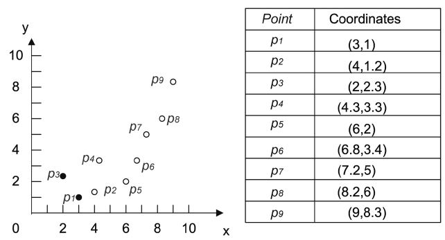
Contemporaneously, the top-k dominating query has also played an increasingly significant role in applications such as multi-criteria decision making, data cleaning, data integration [14] and so on. However, top-k dominating queries are a little different from their skyline counterparts. Given a data set, the data object in a top-k dominating query is not always a skyline of this data set, but it is guaranteed that the top-1 dominating data object must be a skyline. This is because the data object which dominates the largest number of other data objects can’t be dominated by any other data object, so it must be a skyline. Fig. 2 shows an example where nine data points are located in a 2-dimensional space. Assume that a point p dominates another point q when p has smaller coordinates than q in both dimensions. We can observe that p1 and p3 in Fig. 2 are skylines, and that they dominate seven and five points respectively. However, given a top-2 dominating query, we can also observe that p1 and p2 are the top-2 dominating points instead of p1 and p3, the reason being that p1 obviously dominates the largest number of points and p2 dominates the second largest number of points (i.e., six points). This is more than the number of points dominated by p3 (i.e., five points).
Most of the existing works have so far concentrated on addressing how to retrieve the top-k dominating data objects [1-3, 5, 6]. The authors in [6] proposed a skylinebased top-k dominating algorithm (skyline-based top-k dominating, STD) for top-k dominating queries, where the data is indexed by R-tree [15]. It first retrieves the skylines of a data set, and then outputs the skyline (say, o) which dominates the largest number of data objects in this skyline set as the top-1 dominating data object. After this it removes o from the data set and repeats the above process k times. Web services, as a key technique for implementing service-oriented architecture (SOA), have had more and more importance attached to them. With the rapid development of Web services, quite a few services are emerging which provide the same functionality but may differ in the QoS. Therefore, subsequent works have focused on how to select the most desirable service from all functionality-similar services. In [16], a framework to evaluate the QoS from a vast number of Web services is constructed, with an aim to enable quality-driven Web service selection. The proposed QoS computation model includes not only generic criteria (e.g., price, response time, availability, etc.), but also domain specific criteria, which vary with different application backgrounds. The work in [17] mainly focuses on the trust level between service users and service providers. For the reasons that the service users lack enough experience to obtain the best selection of Web services according to its QoS, and that no guaranteed level of QoS can be offered by service providers, they introduce a third party certification entity to verify the conformity of the trust level, as well as the consistency of the QoS claimed by service providers. The authors of [18, 19] propose to employ skyline and top-k dominating techniques respectively to tackle the drawbacks of the traditional method, namely, to require service users to assign weights to each QoS attribute. However, all the above works have considered neither the nature of the Web service environments (i.e., dynamics) nor concurrence. In [20], the authors propose to compute skyline services for Web service composition. In order to reduce computational costs, they preprocess each component service in a composite service. In other words they skip those candidate services in each service which cannot belong to skylines in Web service composition. In order to identify the best candidate semantic Web services given the description of a requested service, the authors of [21] adopt skyline query techniques to solve this problem. In their works, they only focus on the functional part of the Web service, such as inputs, outputs, preconditions and effects. However, the nonfunctional part of Web service (i.e., QoS) also plays an important role in identifying good Web services. Although the work of [22] has taken into consideration the dynamics of the Web services, their judgment on whether a service provider S can currently provide a better service than another provider T is implicitly based only on the corresponding transactions which occurred in the past. Such an implication, however, does not always hold in the very dynamic Web service environments.
In this section, we firstly give a rough description on our service selection scheme. Then we formally describe the top-k dominating query of Web services. Finally we discuss the data structure to be used in this paper for multi-dimensional spatial access.
For some services which are deployed over real-time systems such as real-time ticket ordering services, there may be multiple requests arriving during a small time slot or even at the same time. If these requests are designated to the same service as shown in the motivating example, the performance with regards to some QoS criterion such as response time may degrade. Besides, the composite service is also confronted with another situation, in which a component service provided by some standalone organization in one composite service may be requested by another composite service. These composite services don’t own component services (e.g., these two kinds of services are provided by different providers), and they also need to invoke these component services in line with some service language specification such as Web services business process execution language (WS-BPEL). If we take into account the dynamics of Web service environments, the situation may become more complicated. On one hand, for some standalone component services, they may be invoked at the same time from different composite services; on the other hand, for a composite service, it does not accomplish users’ requests until all of its component services finish. If there are multiple requests arriving or some component service is invoked at the same time by another composite service, then overall performance of the composite service may also degrade. In order to avoid the aforementioned situation, we propose in this paper to select component services in a random manner. Given a user request for a composite service, we first preselect k outstanding candidate services for each component, then we randomly select one candidate service for each component from these preselected services and finally we combine these selected services into a composite service to respond to user’ requests. These works can be accomplished by the service brokers deployed for each service class (i.e., the set of services which have the same or similar functionality). As far as one composite service is concerned, it avoids employing the same candidate service as the traditional service selection scheme does (e.g., s21 and s31 in the motivating example) in response to multiple requests. For some standalone component service invoked by multiple composite services, it also has sufficient power to designate appropriate candidate services to handle the requests passed on from multiple composite services (i.e., faced by multiple user requests). We model our service selection problem as a top-k dominating query problem. In the next section, we describe our problem formulation and then discuss some foundations of the data structure to be used for multi-dimensional spatial access.
Let S be an abstract service class with n services, where each service has d attributes with regards to the QoS. We use si.attrk to denote the k-th dimensional value of the QoS for the service si such that si can be represented as si = < si.attr1, si.attr2,..., si.attrd >.
DEFINITION 1 (Service domination) A service si dominates another service sj if and only if si.attrk?sj.attrk for 1?k?d and there exists at least one dimension λ (1?λ?d) such that si.attrλ > sj.attrλ.
Note that the QoS parameters have different taxonomies reflecting their different perspectives. In [23], the authors distinguished two types of QoS parameters: positive and negative. For a positive QoS parameter, a higher value means higher quality. For a negative QoS parameter, a higher value means lower quality. For example, reliability is positive while response time is negative. In order to make the comparison in Definition 1 unambiguous and uniform, we need to normalize the QoS parameters. Given a service with QoS parameters, we convert the negative parameters into positive parameters using the inverse of the negative parameters. For example, in terms of response time (the negative parameter), a service s1 with a response time of 100 ms is better than another service s2 with a response time of 200 ms. Since the response time of s1 is smaller than that of s2, after conversion, s1 is still better than s2 with regards to response time as the response time of s1 (1/100 ms) is larger than that of s2 (1/200 ms).
PROPERTY 1. If a service si dominates another service sj and sj dominates sk, then si dominates sk. That is, if si?sj and sj?sk, then si?sk.
This property is obvious by Definition 1, so the proof is omitted. Despite its intuitiveness, it is very effective for pruning the search space.
DEFINITION 2 (Dominating score). Given a service s, we can define its dominating score, denoted by ψ(s), as: ψ(s) = |{s'|s?s', s' and s belong to the same service class}.
In order to retrieve the top-k dominating services, we only need to obtain k services whose dominating scores are larger than those of the remaining services. We will detail how to calculate the dominating scores in the next section.
PROPERTY 2. Given two services s and s', if s dominates s', then the dominating score of s is larger than that of s'. That is, s?s'⇒ψ(s) > ψ(s').
PROOF: According to Property 1, s will dominate any service which is dominated by s' if s dominates s'. In other words, the dominating score of s is at least larger than or equal to that of s' plus one, since s dominates s'. Hence, ψ(s) > ψ(s').
However, if ψ(s) > ψ(s') holds, it does not mean that s must dominate s'. Consider points p2 and p3 in Fig. 2. For example, though ψ(p2) (i.e., 6) is larger than ψ(p3) (i.e., 5), p2 does not dominate p3.
Given an abstract service class S with n services which
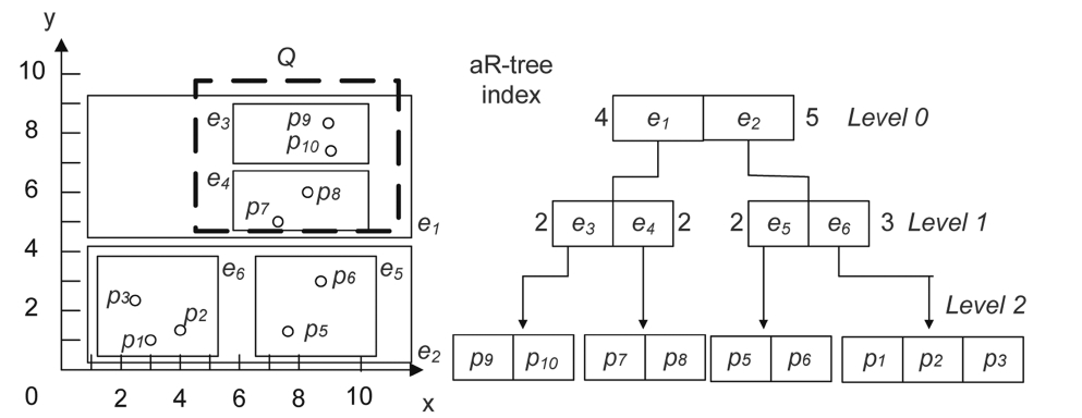
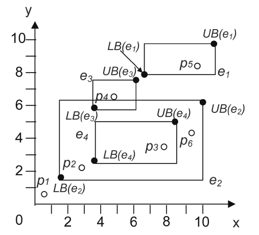
have the same functionality, we want to retrieve the top-k dominating services. Obviously, a naive way to obtain these services is as follows: For each service si in S, we compare it to the remaining services one by one also in S, and obtain the number of services dominated by si. Clearly, this nested loop method is very expensive in terms of both CPU and I/O’s, since it requires quadratic cost with regards to the service class size |S|. A service can be viewed as a d-dimensional data point in terms of QoS attributes. In order to quickly obtain the top-k dominating services, we adopt a multi-dimensional index aRtree [5, 24, 25] over the d-dimensional services in a service class, which can provide faster access to data points than the sequential scan. R-trees have attracted significant attention in spatial databases because they provide effective access methods for multi-dimensional data and for processing spatial queries, such as range queries and skyline queries. The aR-tree, a variant of an R-tree, augments to each non-leaf entry of the R-tree an aggregate measure of all data points in the subtree pointed by it. Fig. 3 shows an example of an aR-tree in 2-dimensional space where each non-leaf entry records the number of data points contained in the subtree pointed by it. For instance, entry e1 in the root node contains four data points tagged with the number “4” around the entry and entry e3 contains two data points. Through the aR-tree, we can effectively and efficiently prune the search space. Assume that given a query Q, we want to find out the number of all data points covered by Q. Firstly, we search the root node and find that entry e1 intersects Q and e2 does not. Then we only need to search the subtree pointed by e1 and can prune away the subtree pointed by e2, the reason being that any data point indexed by the subtree of e2 can not be covered by Q. Finally, we find that both entries e3 and e4 are spatially covered by Q, so data points contained by e3 and e4 must also be contained by Q. The answer (4) to the query can at last be returned by using the aR-tree directly without requiring an inspection of each data point for Q. Before proceeding further, we go through some notations below which will be used later. For an aR-tree entry ei, (i.e., a minimum bounding rectangle (MBR) [5, 15]), we represent it in the j-th dimension using the interval [LB(ei, j), UB(ei, j)], where LB(ei, j) and UB(ei, j) are the lower and upper bounds of ei in the j-th dimension, respectively. We can obtain LB(ei, j) and UB(ei, j) from the projection of ei in the j-th dimension. Therefore, the lower and upper bounds of ei can be represented as:
LB(ei)=(LB(e1,1), LB(ei,2)..., LB(ei,d))
UB(ei)=(UB(e1,1), UB(ei,2)..., UB(ei,d))
Note that both LB(ei) and UB(ei) are virtual (conceptual) data points, which means they do not correspond to actual data points. However, through the lower and upper bounds of an entry, we can better understand the dominance relationship between data points and MBRs. Let us look at Fig. 4 (in the 2-dimensional space) as an example. For the sake of consistency and clear presentation, we make the same assumption that we did in Fig. 2. Therefore, for each entry the lower bound dominates the upper bound, i.e., LB(e1)?UB(e1), LB(e2)?UB(e2), and so on. As can be seen from Fig. 4:
1. There exists no dominance relationship between the entry and a data point. We use ? to denote this no-
dominance relationship, so we have p6?UB(e3) (or LB(e3));
2. If some data point p dominates the lower bound of an entry e (i.e., p?LB(e)), p then must dominate all data points indexed under e (for instance, since p1?LB(e2), p1 must dominate p2 and p3 which are indexed under e2);
3. If some data point p dominates the upper bound but does not dominate the lower bound of an entry, p may then not dominate any data points indexed under that entry (for instance, since p3 dominates UB(e2) and p3 does not dominate LB(e2), p3 can dominate p6, but p3 cannot dominate p2); and
4. If some data point p is dominated by the upper bound of the entry, all the data points indexed under e dominate p (for example, since UB(e3) dominates p5, p4 dominates p5).
In this section, we present aR-tree based algorithms for efficiently computing the top-k dominating services. Assume that the services have already been indexed by an aR-tree, in which all the entries in the leaf nodes record the references to the services.
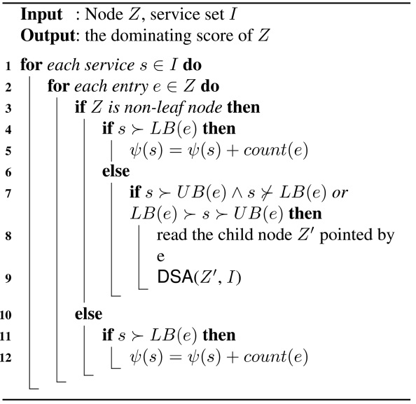
As explained earlier, the naive method is prohibitive due to quadratic cost with regards to the service class size |S|, in terms of both CPU and I/O’s. Instead, we may avoid comparing each service to all other services by using an aR-tree. For example in Fig. 4, if we know that p1?LB(e2), then there is no need to further examine the dominance relationships between p1 and the data points indexed under e2 because it is already known that p1 dominates all data points indexed under e2, according to the lower and upper bounds of entry. The details on how to obtain the dominating score for each service are shown in ALGORITHM 1, called the dominating score algorithm (DSA). This algorithm takes two parameters: the current aR-tree node Z and the service set I, in which the dominating score ψ of all the services will be counted. Note that the elements in I may or may not come from the services which are indexed by the aR-tree denoted by the first parameter. For instance, the set I sometimes consists of lower and upper bounds of entries, as will be discussed later in our next algorithm.
Recall that there are four cases of dominance relationships between an entry e and other services (ref. III-C). In our approach, we aim to find out the services which dominate LB(e) (assume that LB(e)?UB(e)) when entry e is examined. As for those services which are dominated by UB(e), the dominating scores of them can not be calcu-
lated with the help of e. Initially, Z is set to the root node of the tree and ψ(s) is set to 0 for each service s∈I. Let e be the current entry in Z to be examined. For each service s∈I, we traverse the aR-tree to find out how many services indexed by the aR-tree are dominated by s (i.e., ψ(s)). If e is a non-leaf entry (line 3) and the s which is currently being examined satisfies the condition of s?LB(e), then we increase the dominating score of s by COUNT(e) which is the number of services indexed under e (lines 4-5). If e is a non-leaf entry and the dominance relationship between e and s belongs to one of the two cases where (1) s?UB(e) and s?LB(e), or (2) s?UB(e) and LB(e)?s, then s may dominate some services indexed under e. However, this cannot guarantee that s will dominate all of the services indexed under e, since there does not exist a dominance relationship between s and LB(e) in (1), and even with LB(e)?s in (2) there still does not exist exact dominance relationships between s and the other services indexed under e. Take Fig. 3 for example. Let s be p1 and e be e6, respectively. We can see that s?UB(e) and LB(e)?s, but we still do not know the exact dominance relationship between s and p2 (or p3) without comparing them. Therefore, it is not easy for us to immediately deduce the number of services in e dominated by s. In this situation, we need to invoke the algorithm recursively on the child nodes pointed by e (lines 8-9). Lastly, if Z is a leaf node (i.e., e is a leaf entry), we just need to increase the dominating score of any service that dominates LB(e) by COUNT(e) (line 12).
Note that DSA can correctly calculate the dominating scores ψ for all services s∈I through a single traversal of the tree. Suppose that component services are already indexed by an aR-tree as in Fig. 3, where the data points represent the services. The service set I is composed of p1, p2, and p3. Now we calculate the dominating scores of the services in I step by step. According to DSA, for p1, entry e1 should first be examined, and e3 is then next, due to the fact that p1?UB(e1) and p1?LB(e1). Because p1 dominates LB(e3), the dominating score of p1 (i.e., ψ(p1)) is increased by COUNT(e3) (i.e., 2). Then e4 is examined, and ψ(p1) is increased by COUNT(e4) since p1 also dominates LB(e4). When e2 is examined, DSA will recursively examine its child node entries, i.e., e5 and e6, respectively, due to the fact that p1?UB(e2) and p1?LB(e2). When e6 is examined, since LB(e6)?p1?UB(e6), DSA will examine the child node pointed by e6. The child node is a leaf node, so the dominance relationships between p1 and other services (i.e., p2 and p3) are examined by comparing them with p1. The situation can be handled similarly when the entry e5 is examined. Therefore, the dominating score of p1 can be counted correctly. Finally, p2 and p3 can also be counted correctly in the same way as p1 was.
Note that we can obtain the top-k services by using only DSA, because after the score for each service is calculated, we just need to select the k services whose dominating scores are larger than the others’. However, if the number of services is very large, say, thousands of services in I, it is quite time-consuming to calculate the dominating scores, as the algorithm needs to exhaustively check all services in I each time. To avoid such a situation, we present below a depth first retrieving (DFR) algorithm, as shown in ALGORITHM 2, with the aim to greatly reduce the number of services in I when calculating the dominating scores. In particular, we adopt the idea proposed in [3] by using the data points which have been pruned to further prune the search space, and combine it with DSA to retrieve the top-k services. When traversing the entries from the root node of the tree denoted by “R.root” in Algorithm 2, we employ a max-heap H to store the dominating scores of the lower bounds of entries in the current node (line 5). By doing this, we can preferentially search and calculate the services which dominate more services than others do (lines 7-8). In order to further prune the search space, a list

is maintained, to store the pruned services and their corresponding dominating scores. Specifically, the services in
are not dominated by each other. If there exists some service I in
, such that l dominates the lower bound of entry e, then we do not need to check the services indexed under e, and can thus abandon e directly without putting it into H. This is because according to Property 1, all the services indexed under e are dominated by l. When extracting the top entry from H and beginning its traversal, we employ another condition to control the repetition (line 6), in addition to checking whether H is empty. The variable ρ represents the k-th highest dominating score which has been found so far. If the top entry’s dominating score
from H is lower than ρ, we can stop extracting entries from H. Finally we maintain a min-heap h that stores the top-k dominating services. Note that h,
and ρ are updated in time after the indexed services are traversed (lines 16-33).
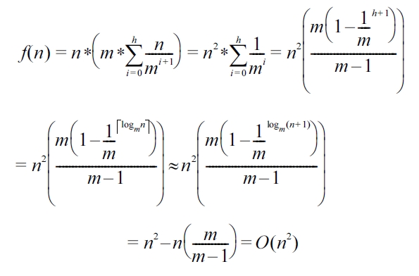
We can retrieve the top-k dominating services by both DSA and DFR. However, there exist some differences in terms of their performance. In this subsection, we analyze and compare the two algorithms with regard to time complexity. In finding the dominating score of each service in a given service set, we note that both DSA and DFR in essence traverse the aR-tree node by node. Nevertheless, the differences lie in that. On the one hand, DSA just obtains the dominating score of each service in a given service set without directly fetching the top-k dominating services and it must further cooperate with a sorting algorithm to gain the desired services, while DFR can obtain the top-k dominating services directly. On the other hand, when DSA is used alone, the second parameter (i.e., the service set I) should contain all the services which are indexed by the aR-tree. The outer for-loop (line 1 in DSA) therefore will incur relatively large computational overheads. Let the aR-tree nodes have an average fanout m, i.e., the number of entries in one node. Suppose that the number of services which are indexed by the aR-tree is n. Then the tree height h can be estimated by h =
and the number of nodes ni at level i (with the leaf level being zero) can also be estimated by ni = n/ mi 1. We use T(n) = O(f(n)) to represent the time complexity of DSA and DFR. For each service s from the service set I, the worst case scenario of DSA is that s needs to be compared with every entry in the aR-tree. Therefore, f(n) can be represented as follows:
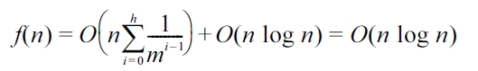
However, in DFR, we can have:
where, O(n log n) denotes the time complexity of the heapsort algorithm used to sort the entries and retrieve top-k dominating services (ref. line 7 and line 21 of Algorithm 2). Accordingly, when the number of indexed services is very large, DFR has an obvious advantage over DSA.
In this section, we demonstrate the efficiency and effectiveness of our approach by conducting extensive experiments. In the first experiment, we study the relationships between response time and the workload of the service server. Then a series of experiments are conducted to verify the advantages of our approach over baseline and traditional methods for service selection when responding to a large number of concurrent requests. Finally we study the influences of certain parameters over our service selection scheme, including the size of the service class, the number of service classes in a composite service and so on.
We run our experiments on a PC with a 2.2 GHz Intel Pentium Duo2 CPU, 2,048 M of RAM, Microsoft Windows XP Operating System, J2SDK 1.6. It is worth noting that the aR-tree we use to index services is completely dynamic [15], which mean that inserts and deletes are intermixed with searches and no periodic reorganization is required. All the services are pre-indexed by an aR-tree structure before they start responding to any requests.
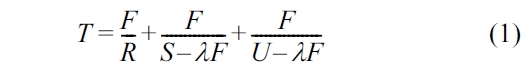
As we discussed earlier, the QoS attributes of services may sometimes degrade due to the overload of servers and the dynamics of Web service environments. According to the M/M/1 model and the method proposed in [26], we can estimate the average response time as follows:
where,
F: average file size
R: client network bandwidth
λ: network arrival rate
S: server network bandwidth
U: file read rate
Formula (1) indicates that with the increment of the network arrival rate (i.e., λ), the average response time from a Web server also increases. However, this cannot be directly applied to obtaining the average response time for Web services because the response time denoted in this equation usually means the round trip time of getting some files which are stored on the Web server (rather than the service server), such as videos or audios contained in Web pages. Nevertheless, we still get the idea from the equation that the average response time from a service server could increase sharply if the number of concurrent requests increases. To the best of our knowledge, there is no existing work which elaborates on the relationship between the response time and the workload of the Web service server. In order to analyze this relationship fairly and objectively, we conducted the first experiment by examining the performance of a general real-life service with regards to its response time under a differing number of concurrent requests.
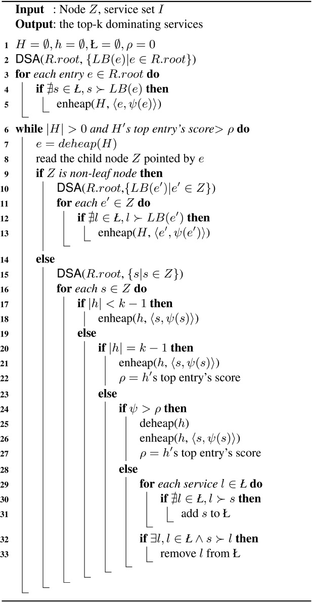
Fig. 5 shows the variation in the average response time for a service with different numbers of requests. Given a request, the normal (advertised) response time of the service we choose is within and around 100 ms in this experiment. As can be seen from Fig. 5, although the average
response time of the given service approximates in a linear fashion as the number of concurrent request increases, the curve takes on two different variations with the increasing number of concurrent requests. For instance, when the number of concurrent requests varies between 10 and 60, the average response time increases slowly. This is because other requests should wait in line while the current request is being accomplished so the capabilities of the service server do not reach beyond maximum. However, when the number of concurrent requests exceeds 60 and continues to increase, we can see that the response time increases very fast. This is because large quantities of concurrent requests result in the overload of the service server, which gives rise to the fluctuation of the overall performance for the provided service, and usually this fluctuation turns into QoS degradation such as longer response time. In other words, in this experiment the capabilities of handling 60 concurrent requests almost creates a workload bottleneck in the service server.
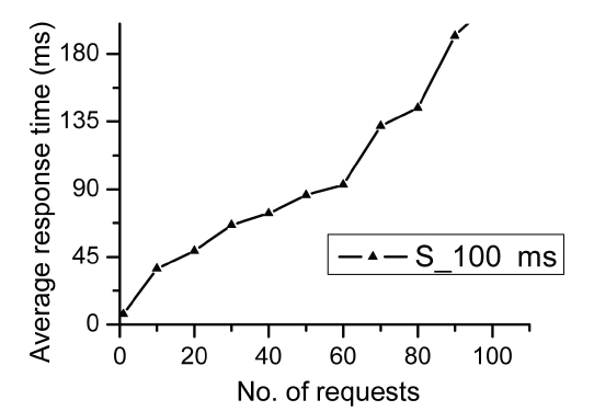
In our next set of experiments, we evaluate the performance of our composition approach by comparing it with two other methods. One is the traditional method based on a utility function (UF) as described in Section I and the other is the random method as the baseline. In our approach, we first use the algorithm DFR to obtain top-k services for each component service of a composite service. For an incoming request, a composition solution which consists of services randomly chosen from top-k dominating services from each component service class is created to respond to the request. In the traditional method, the composition solution having the maximum value of UF is always chosen and designated for responding to the request. The random method, however, always selects a composition solution that consists of services randomly chosen from each component service class, as opposed to being chosen from top-k dominating services. First, we design a composite service which comprises several component services. In the next experiments, we study the influences of the number of component services
in a composite service as well as the number of candidate services in a service class over our service selection scheme. In this subsection, we assume that the composite service includes four component services, and each component service contains 10,000 candidate services. Then we employ the aR-tree structure to index these services. We conduct the following experiment afterwards. In particular, we employ different composition solutions (i.e., top-k, traditional and random) to respond to the incoming concurrent requests. Fig. 6 shows the performance comparison amongst the three methods. Note that the X-axis represents the number of concurrent requests where the maximum number of such requests is 300. The Y-axis represents the average response time for each service selection scheme. We set the value of the variable k to 2, 5, 10, and 50, respectively, in order to thoroughly study the performance of our approach under different values for k. For both our approach and the traditional method, when the number of concurrent requests increases, the average utility value (with respect to the average response time) also becomes larger, which conforms to the result from Fig. 5. As for the random method, the performance is not stable, as the QoS of services chosen randomly is uncertain. We also observe that no matter which value the variable k is set to be, our approach always performs better than the traditional method. Compared to the traditional method it is useful to observe that the advantage of our top-k approach is even more apparent when the number of concurrent requests increases. Meanwhile, we can also see that the performance of our approach improves as the value of k increases. Nevertheless, it does not always mean that the higher the value of k, the better the performance of our approach. This is because the overheads of our approach include not only the response time (incurred from performing the requests), but also the cost of retrieving the top-k dominating services.
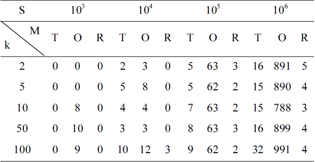
The latter however depends on the number of candidate services in each component service class. Although we can retrieve the top-k dominating services off-line, it is only fair to take this part of our overheads into account when comparing our approach with the others objectively. Table 1 shows different overheads on time (measured by “ms”) under different numbers of services in a service class. Note that in Table 1, “T” denotes the traditional selection method, “R” denotes the random selection method and “O” denotes our approach. In order to ensure the fairness and accuracy of our measure, given a different number of services, we run each of the three methods under different k values 1,000 times, and then we obtain the mean time overheads for each method. We can observe that for our approach no matter which value k is, when the number of services in the service class increases the corresponding overhead also increases. This is because DFR (ALGORITHM 2) which is employed to retrieve the top-k dominating services is not independent of service class scale. When the service class scale is settled and the number of services is not so large (say, 103, 104 or 105), the overhead of our approach is almost the same as that of the other two methods. When the number of services is very large (e.g., 106), the difference in terms of overheads between our approach and the other two methods becomes more notable, even though the results are still acceptable in practice. To the best of our knowledge, there exist few service classes which contain more than 105 services in most real-life applications. Also, we can retrieve the top-k dominating services off-line so that we only need to re-calculate the top-k dominating services when the information about the QoS needs to be updated. From Table 1, we can also see that the random
method takes almost the same amount of time when compared to the other two methods, whether the number of services increases or not. This is expected since the random method chooses k services from each service class randomly, for which the time complexity is O(1).
In this subsection, we turn our attention to three parameters which have some influence over our approach. In particular, we take into account the parameters of service class size (i.e., the number of candidate services in a service class) denoted by SSize, the number of service classes in a composite service (denoted by CSize), and the value k denoted by top-k, respectively. In order to study the effects of these parameters, we conduct three sets of experiments, where we fix two of the parameters and then vary the remaining one. To fix the parameters (i.e., SSize, CSize, top-k), we set the default values to 1,000, 4, 10, respectively.
1) top-k
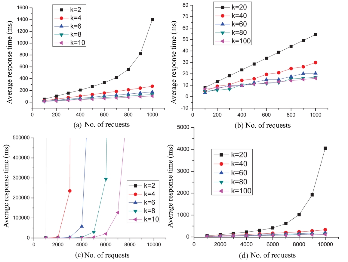
To study the impact of the top-k approach, we have conducted a series of experiments with different scales in terms of the number of concurrent requests. Namely, we vary the number of concurrent requests between 100 and 103 with a step value of 100, and between 103 and 104 with a step value of 103, respectively. The corresponding values of SSize and CSize are the default values. Fig. 7 shows the experimental results. Specifically, Figs. 7a, b depict the variations in the average response time under different values for k when the number of concurrent requests vary between 100 and 1,000; Figs. 7c, d depict the variations in the average response time under k when the number of concurrent requests vary between 103 and 104. The experimental results show that: 1) For each curve (i.e., with a fixed value of top-k), the average response time becomes larger when the number of concurrent requests is increasing. 2) As the value of top-k increases, the performance of our service selection scheme generally gets better, although it does not mean that the larger the value of top-k, the better our performance. This is because the overhead on retrieving top-k services in each service class is not negligible, especially when the value of top-k is considerably large. As a matter of fact, we found in our experiments that given the number of concurrent requests, the preferable value of top-k does not always correspond to the largest value of k. For instance, as denoted in Fig. 7b, with the number of concurrent requests varying between 100 and 103, the performance of our service selection scheme is almost the same when the value of top-k is set to 80 and 100, respectively.
If we take into account the overheads on retrieving the top k services, the performance when the top-k = 80 is obviously better than that when the top-k = 100. 3) If the value of the top-k is set inappropriately with respect to the number of concurrent requests, the performance can be unfavorable. As shown in Fig. 7c, when the number of concurrent requests varies between 103 and 104 and the value of top-k is set to 2, 4, 6, 8, and 10, respectively, we can see that the overheads are considerably larger compared to the overheads shown in Fig. 7d where the value of top-k is set to 20, 40, 60, 80, and 100, respectively.
2) SSize
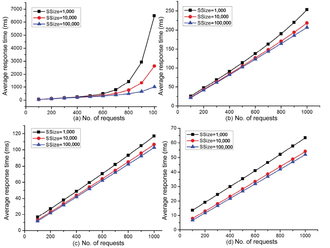
SSize indicates the number of candidate services in a service class. To study the impact of SSize on the performance of our approach, we have also conducted a series of experiments where we vary the number of concurrent requests between 100 and 1,000 with a step value of 100. In each experiment, we compare the performance of our approach for three different values of SSize, namely; 103, 104, and 105, respectively.
The experimental results are shown in Fig. 8. The only difference between these experiments (denoted by Fig. 8) lies in the values of top-k. For example, we set the values of top-k in Fig. 8 to be 2, 5, 10, and 20, respectively. From these figures, we can observe that: 1) for each curve (i.e., the number of candidate services in one service class is fixed), when the number of concurrent requests grows, the response time of our approach also increases. Besides, the performance degradation in terms of response time does not always decrease in a linear fashion as the number of concurrent request increases. Take Fig. 8a for instance. When the number of concurrent requests reaches 800, the performance of our approach begins to degrade sharply, regardless of the values of SSize. 2) When the value of SSize becomes larger, the performance of our approach also improves with regards to the response time. In Fig. 8a, for example, when the number of concurrent requests is within 500, no matter what the value of SSize is set to, the performance of the service selection scheme is almost the same. However, with the number of concurrent requests continuing to grow, the service selection scheme with SSize = 105 is much better than that with SSize = 103 or 104. Meanwhile, the service selection scheme with SSize = 103 behaves the worst when compared to the other two service selection schemes with a smaller SSize. Since the services in our experiments are generated randomly, the QoS for each candidate service is also uniformly distributed. Whether we can select (relatively) good Web services in terms of QoS actually depends on the cardinal number, i.e., SSize. This is because the larger the value of SSize, the higher
the probability that a service class may contain good candidate services which can be obtained by using the top-k dominating technique. As reflected by the experiments in Fig. 8, however, we also find that when SSize is extremely large, the overhead on retrieving top-k candidate services also becomes prohibitive. Consequently, there should be a balance between the performances of the selection scheme and the overheads on retrieving the top-k candidate services. According to previous experience and our experiments, SSize with the value of 104 is sufficient to demonstrate the effectiveness of our approach. As mentioned before, there are few service classes which contain more than 105 services in most real-life applications. 3) When the value of SSize is fixed at say 105, the performance of our service selection scheme in Fig. 8d is much better than that in Fig. 8c.
The difference on the performance can be easily distinguished, because the value of top-k in Fig. 8c is 10, while in Fig. 8d the value of top-k is 20. From this set of experiments, we can observe that as the value of top-k increases, the performance of our service selection scheme also improves to some extent.
3) CSize
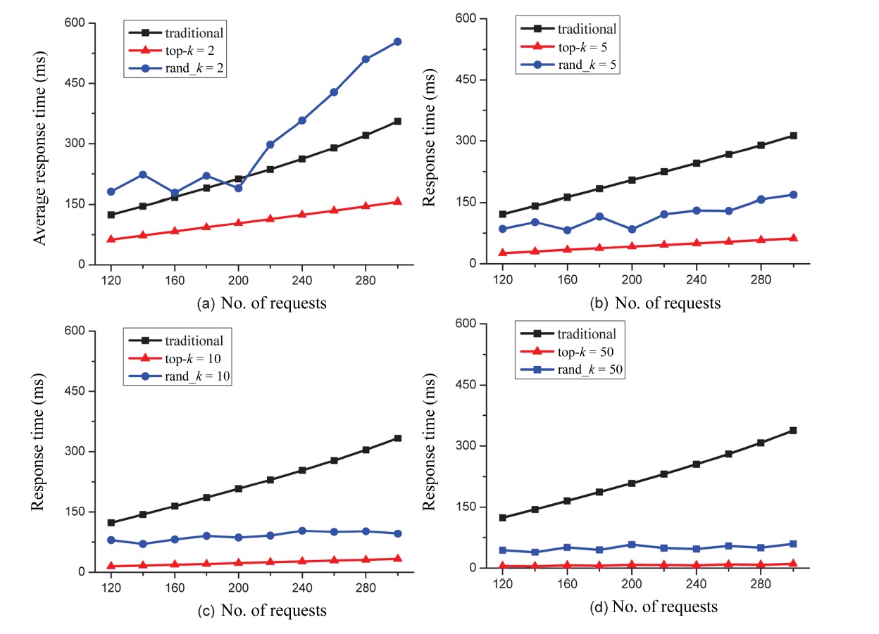
CSize denotes the number of component services in a composite service. In this set of experiments, we study CSize over the performance of our approach. We vary the number of concurrent requests (denoted in X-axis) between 100 and 1,000 with a step value of 100. In each experiment, we analyze the performance of our approach with regard to the average response time for each service class under five different values of CSize, i.e., 2, 4, 6, 8, and 10, respectively. The experimental results are shown in Fig. 9. Note that the only difference among these experiments (denoted by Fig. 9) lies in the values of top-k. In particular, the value of top-k in Fig. 9a to Fig. 9d is set at 2, 5, 10, and 20, respectively. The value of SSize in this experiment is set to 104. From the results, we can see that: 1) With the number of concurrent requests increasing, no matter which value CSize is, the average response time also increases. This variation actually complies with the development trend reflected in the previous experiments. 2) When the number of concurrent requests is fixed, the average response time of our approach under different values of CSize is in fact, almost the same. The reason is that the component services in a composite service are generated randomly, which means that each component service of the composite service exhibits similar behavior. Overall, we can see that the total response time for the composite service increases proportionally to the growth of the number of component services in a composite service. Furthermore, the average response
time for each service class in a composite service stays almost the same. Thus, we can see from this set of experiments that CSize has little influence over our service selection scheme.
In this paper, we have presented a service selection scheme which adopts top-k dominating queries to generate a composition solution. In particular, to handle a given request, we select the composition solution by adopting a top-k dominating query technique for each component service. Through extensive experimentation, we have verified the efficiency and effectiveness of our approach in comparison to the baseline and traditional service selection schemes. For future work, we plan to further improve the overall performance of DFR and balance the overheads between retrieving the top-k dominating services and the top-k service selection scheme.