Steady solutions of fluid flows can be obtained by solving the Euler equations, or the Navier-Stokes equations, with time marching methods. The time marching methods, however, are not applicable to the incompressible Navier-Stokes equations because the continuity equation has no time derivative, unlike the momentum equations. To overcome the difficulty associated with the lack of the continuity equation, Chorin (1967) proposed an artificial compressibility method where an artificial time derivative term of pressure is added to the continuity equation with an artificial compressibility parameter (
After Chorin’s pioneering work, many researchers applied the artificial compressibility method to various incompressible flow analyses. Peyret and Taylor (1983), and Rahman and Siikonen (2008) solved the steady flow problems using the artificial compressibility method. Merkle and Athavale (1987), and Rogers and Kwak (1990) analyzed unsteady flows using the dual time stepping method with the artificial compressibility method. Turkel (1987) suggested a modification of the artificial compressibility method, where artificial time derivatives are added to the momentum equations as well as the continuity equation. This modification introduced an additional parameter (
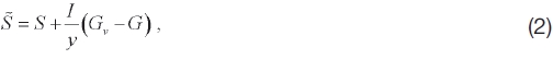
Most research concerned with the modified artificial compressibility method has so far been based on the central difference method with the 2nd order and the 4th order artificial dissipation. Only a few studies adopted upwind methods for the artificial compressibility method. Pan and Chakravarthy (1989) pointed out that the solution with an upwind method was no longer independent of the artifi cial compressibility parameter, and the built-in dissipation associated with the upwind method could contaminate the solution. However, they argued that accurate solutions could be obtained for a suitable choice of
The objective of this paper is to investigate convergence characteristics of the modified artificial compressibility method with an upwind method. To achieve this, an analysis code is developed based on Roe’s approximate Riemann solver. The following section contains the numerical method used in the paper. Also, Eigenstructure of the incompressible Navier-Stokes equations with the modified artificial compressibility method is given in details. Next, the accuracy and the convergence rates of various incompressible flows are compared. The convergence characteristics with combinations of the two parameters are also examined. In the numerical simulations, the Courant-Friedrichs-Lewy (CFL) number is kept constant in order to exclude eff ects of the CFL number on the convergence characteristics. Conclusions will be drawn from the numerical investigation.
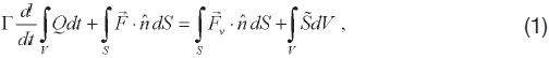
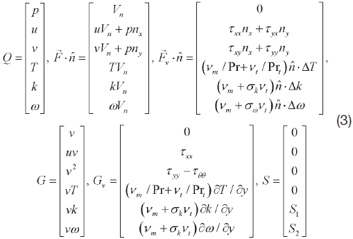
The axisymmetric Reynolds averaged Navier-Stokes (RANS) equations and two equation turbulence model equations for the incompressible flows are chosen as the governing equations. The modified artificial compressibility method of Turkel is adopted in order to use a time marching method. The non-dimensionalized governing equations are as follows:
where

and

are the inviscid vector and the viscous flux vector respectively. The source term,

is defined by:
where

represents the outward normal vector of the computational cell. All of the vectors are defined as
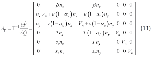
where

where
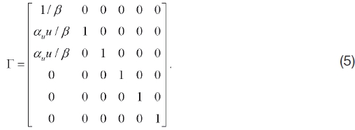
In Eq. (5), the artifi cial compressibility,
The cell-centered fi nite volume method is applied to Eq. (1). The semi-discretized equation is found to be:
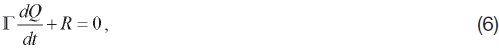
where the residual term is defined as

The total flux vector,

is defined as follows

In Eq. (8),

and

represent the inviscid and viscous flux vectors respectively. The viscous flux vectors are evaluated with the gradient theorem, which is equivalent to the central difference in the Cartesian coordinate system. Th e inviscid flux vectors are computed with Roe’s approximation Riemann solver (Roe, 1981). The numerical flux vector of Roe’s method is given by:

where Δ

and

represent the flux computed using the right state,

is defined by:

The Jacobian matrix,
The eigenvalues of the preconditioned system (1) are found to be:

where


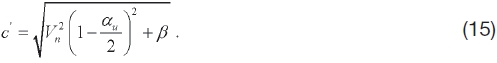
From Eq. (12)-(15),

where

The modal matrix is defined by:
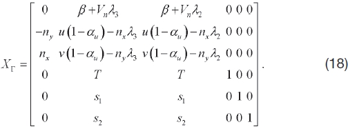
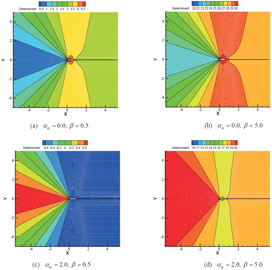
Th us, the determinant of

Equation (19) indicates that the determinant can be zero when

Turkel (1987) derived the same expression as Eq. (20) from the symmetrizability requirement of the system. When central difference methods are used, this manifests as loss of robustness, which was observed by Malan et al. (2002a, b). Most boundary condition methods use characteristic information to determine the solution variables along the computational boundaries. When the determinant of
For the time-integration method, the approximated factorization-alternate direction implicit method (Beam and Warming, 1982) is employed. Detailed information of time discretization can be found in Beam and Warming’s study.
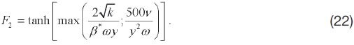
Menter’s
where the blending function,
Other details of the parameters and source term of the
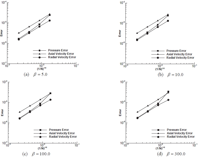
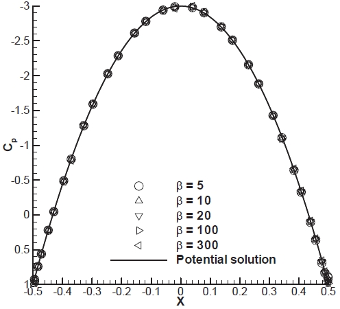
3.1 Inviscid flow around a circular cylinder
As the first computational example, an inviscid flow around a circular cylinder is calculated. This test case is chosen to verify the accuracy of the upwind method and the grid convergence of the modified artifficial compressibility method in conjunction with the upwind method. The
simulations are performed,increasing grid size in variation of
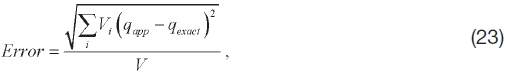
where
[Table 1.] Grid size used for circular cylinder
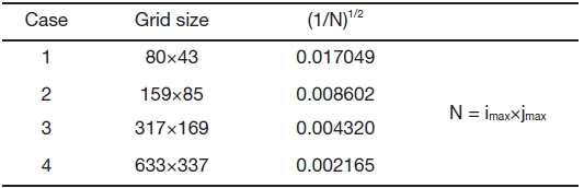
Grid size used for circular cylinder
the accuracy of the solution is guaranteed when a converged solution is obtained (Lax equivalence theorem). Moreover, Roe’s method satisfies the consistency when applied to the artificial compressibility method. The numerical dissipation for the first order upwind method for the Cartesian coordinate system can be expressed as:
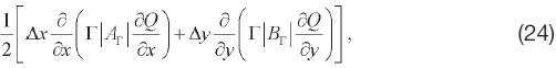
where
From Eq. (24), it is clear that the numerical dissipation vanishes as Δ
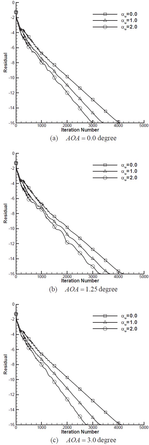
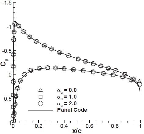
3.2 Inviscid flow around a NACA0012 airfoil
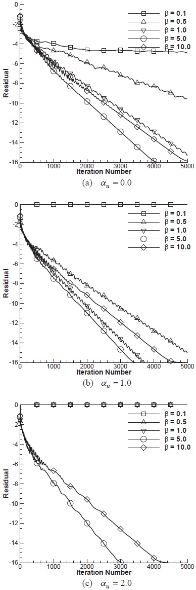
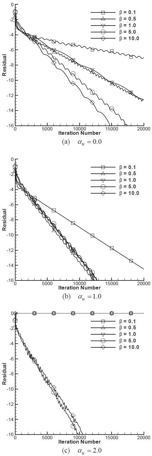
To compare convergence rate with the combinations of
The convergence histories with various
the figure, it is clear that there exists an optimal value for convergence. For this case,
the optimal values of
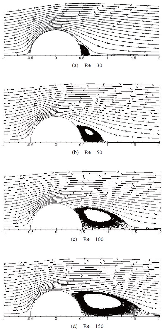
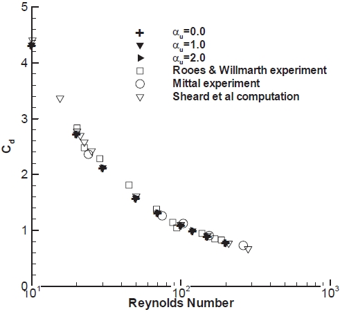
3.3 Laminar flow around a sphere
The second example of examinining convergence characteristics is a laminar flow around a sphere. It is wellknown that flow around a sphere is steady and axisymmetric when Re<220. However, the flow becomes unsteady and
three-dimensional when Re>220. In this paper, numerical simulations are performed with Reynolds numbers less than 220. An O-type computational grid of 129× 57 is used for the computations. The CFL number is set to 3.0 for all computations. Figure 7 depicts the streamlines around the sphere at four different Reynolds numbers; 30, 50, 100, and 150. The size of the separation bubble behind the sphere increases commensurately to the Reynolds number. The drag coefficients computed with different values of
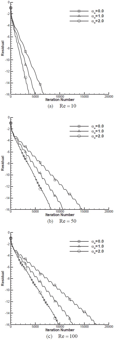
Figure 9 depicts convergence histories of the sphere problem with various combinations of
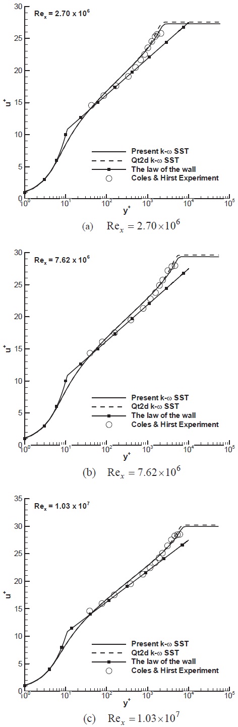
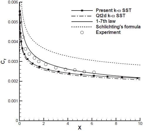
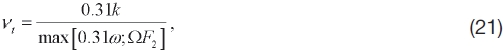
A turbulent flow over a flat plate flow is selected to study the convergence characteristics of the modified artificial compressibility method for turbulent flows. The size of the computational grid is 111×81. The first grid spacing above the wall satisfies the requirement of y+<1 so that the turbulent boundary layer can be correctly resolved. For all the computations, the CFL number of 5.0, the preconditioning factor,
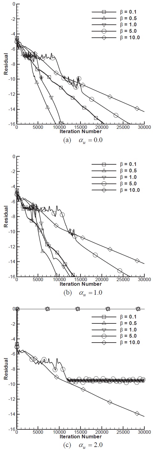
In Fig. 13, convergence histories are compared for the combinations of
the optimal value of
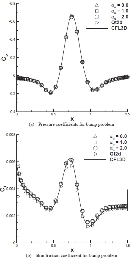
3.5 Turbulent flow passing over a bump
As the final example, the turbulent flow over a bump is selected. This example is one validation case of turbulence
modeling resource at the Langley Research Center website. A grid of 353×161 is downloaded from the website and used for the computation. The first grid spacing above the wall satisfies the grid resolution requirement of
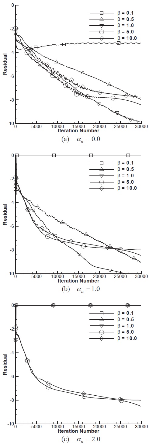
Figure 15 represents convergence histories with combinations of
In this study, an incompressible RANS code, which uses the modified artificial compressibility method of Turkel and the upwind method of Roe, was developed; the convergence characteristics were studied for various incompressible flow problems. It is confirmed numerically and analytically that the accuracy of the solution can be assured with the upwind method and the artificial compressibility method. The modified artificial compressibility method has superior convergence characteristics compared to the original method. However, the modified artificial compressibility method with