Pointing stability of high precision observation satellites is affected by the dimensional stability of the structure [1] and the on-board vibrational disturbance [2]. Transmission of the residual vibration that results from the actuation of various sources such as reaction wheel assembly (RWA), control moment gyroscope (CMG), thrusters, cryocoolers, solar array drives, etc., may prove critical for the operation of sensitive optical payloads. Therefore, in-orbit vibrational environment and its effects on the performance of the optical payload must be predicted and analyzed in design phase in order to ensure that the established requirements on the payload are fully met. In order to achieve this, integrated modeling of disturbance, structure and optical system is preferred.
Previous works in the integrated modeling of optical systems have resulted in the development of Integrated Modeling of Optical Systems (IMOS) toolbox [3], Modeling and Analysis for Controlled Optical Systems (MACOS) software [4], Dynamics- Optics-Controls-Structures (DOCS) toolbox [5] and Integrated Telescope Model (ITM) software [6]. These tools have been used in various missions that include Space Interferometry Mission (SIM) [7], Next Generation Space Telescope (NGST) [8], Thirty Meter Telescope (TMT) [9] and Very Large Telescope Interferometer (VLTI) [10], Terrestrial Planet Finder (TPF) [11] and so on. In this paper, development of an integrated analysis framework has been introduced and it includes the on-board disturbance, structure and optical system model. The purpose of the developed framework is to evaluate the performance of optical payloads in the presence of micro-vibration. Moreover, vibration isolator model is also integrated to analyze the effectiveness of using a vibration isolator for the performance enhancement of optical payloads.
2. Integrated Simulation Tool for Jitter Analysis
2.1 Reaction Wheel Induced Disturbance Modeling
Vibrational disturbances onboard a satellite are generated during the operation of actuators which are used in the attitude control such as RWA, CMG and thrusters. Among these sources of disturbance, RWA is generally known to be the largest source of unwanted vibrational disturbances. A typical component of RWA is a flywheel and it is suspended on a brushless DC motor and bearings. Based on the principle of conservation of angular momentum, control torque is produced as the rotating flywheel is accelerated or decelerated. During the operation of RWAs, apart from the desired control torque, unwanted disturbances due to flywheel imbalance, bearing irregularities and motor imperfections are also generated [12]. In general, disturbance due to the flywheel imbalance is the largest, and its amplitude is proportional to the square of the rotating wheel speed and its frequency is identical to that of the rotating wheel speed. Bearing and motor imperfections result in disturbances that are at both sub- and super- harmonics of the rotating wheel speed [13]. Thus, the frequency content of the disturbances from RWA is not only confined to the rotating wheel speed, but it also comprises of various harmonic components. As mathematical modeling of a reaction wheel with bearing irregularities or motor imperfection is impractical, the induced disturbances are modeled empirically based on the disturbance measurement test. Data from the measurement tests show that the RWA induced disturbances closely match the form that is given in equation 1 in most of the wheel speeds which are outside the vicinity of the wheel’s natural frequency [13]. In equation 1, m(t) is the disturbance (force or torque), C is the amplitude of the disturbance, Ω is the
wheel speed, h is the harmonic number and α is the phase, which is assumed to be random. The coefficients, C and h that characterize a particular disturbance can be obtained by using curve fitting or optimization method using the experimental data.

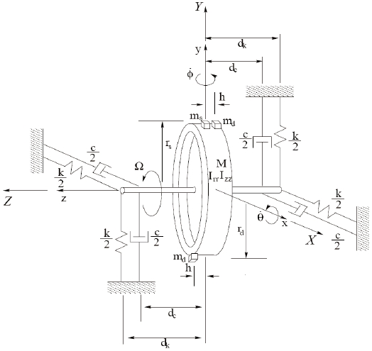
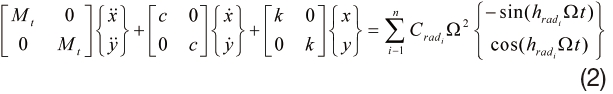
One major limitation of the disturbance model represented by equation 1 is that it cannot represent the resonance phenomenon near the natural frequency of the RWA. This is corroborated by using the test data which shows a very high amplification of disturbance magnitude when the frequency of the induced disturbances matches the natural frequencies of the reaction wheel. As the design phase must also consider the worst case scenarios, it is important to incorporate into the RWA disturbance model the amplification phenomenon due to resonance. The structural resonance effects of RWA induced disturbances can be incorporated by using an analytical model of RWA. Fig. 1 shows the reaction wheel with an imbalance that is used for the analytical model. By assuming that the masses responsible for the imbalance are much smaller compared to that of the total mass, i.e.,
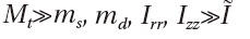
where
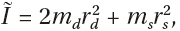
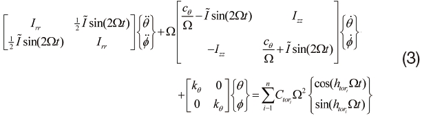
the translational and rotational equations of motion can be approximated as equations 2 and 3, where c, k, cθ and kθ are the damping, stiffness, torsional damping and torsional stiffness of the wheel, respectively [13].
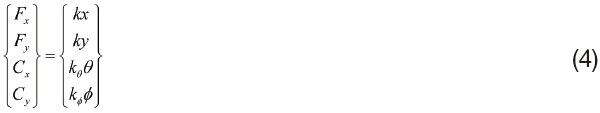
RWA induced disturbances including the resonance phenomenon can be approximated as the transmitted disturbance in the form of equation 4. Here, x, y, θ and ø are obtained by solving for the particular solutions of the equations 2 and 3 by using the disturbance model that is given in equation 1 as the external force and moment. Due to the symmetry of the wheel model, the x and y direction forces (θ and ø direction torques) differ 90 degrees in phase, but they are the same in all the other aspects.
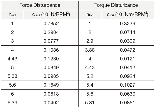
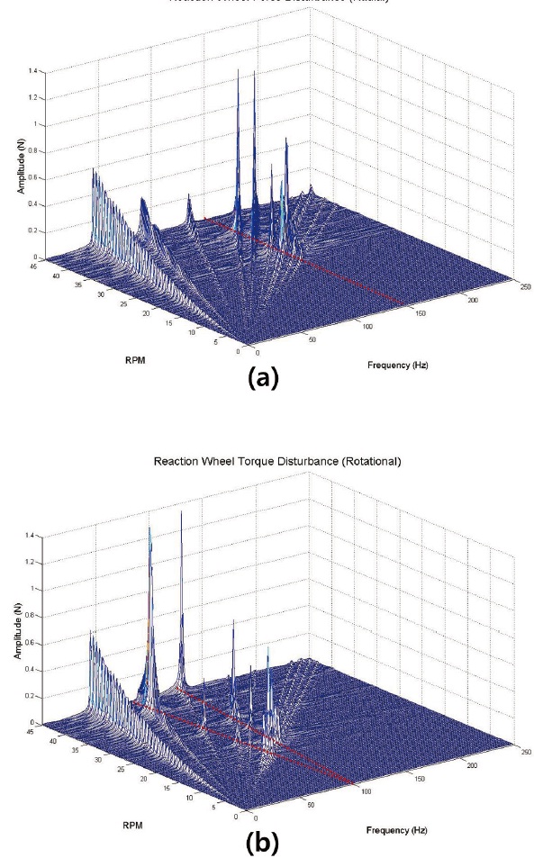
In this study, a reaction wheel’s structural properties (Table 1) and disturbance characteristics (Table 2) are adapted from the numerical model that was developed by Kim, et. al [14]. By using equations 2, 3 and 4, the reaction wheel induced disturbance is generated and it is plotted in Fig. 2. The red dotted lines in the figure indicate the natural frequencies of the wheel. In the translational mode, the natural frequency is constant at 150 Hz, but that of the rotational mode varies along with the wheel speed and it is divided into nutation and precession mode. As the disturbance frequency crosses the natural frequency of the wheel, a huge amplification in the disturbance magnitude is observed.
2.2 Modeling of the Structure in State Space Modal Form
In this study, the structure was modeled by using FEM and modal analysis. Modal analysis is a renowned method for analyzing lightly damped structures. In modal analysis, coupled set of equations in physical coordinates are transformed to uncoupled set in modal coordinates by using eigenvalues and eigenvectors of the system. Here, each uncoupled equation corresponds to a particular mode of vibration. The overall system response can be obtained by summing up the response of individual modes and the
[Table 1.] Structural properties of the reaction wheel model.
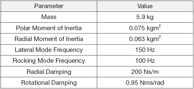
Structural properties of the reaction wheel model.
[Table 2.] Disturbance characteristics of the reaction wheel model.

Disturbance characteristics of the reaction wheel model.
solution in the modal coordinates can be transformed back to the physical coordinate. By transforming FE model to modal model for analyzing the system response can result in the reduction of the computation cost as the number of modes to capture the essence of the system is lesser compared to the number of nodes that are required to model the system.
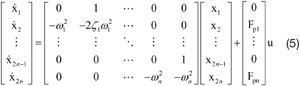
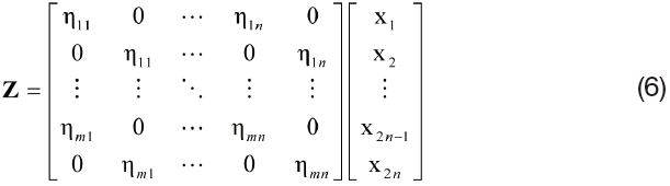
By following the method that was described by Hatch [15], FE model of the structure was built in commercial FEM software ANSYS and it is used to extract the natural frequency and mode shape information of the structure. By using the obtained modal information, modal model of the structure in state space form of equation 5 is created in MATLAB where, the response analysis is conducted. In equation 5, x1, ..., x2n are the displacement of modes, ωi is the ith natural frequency, ζi is the critical damping ratio of the ith mode and Fp1...Fpn are the forces in the modal coordinates. The results in modal coordinates can be transformed back to the physical coordinate through equation 6, where ηij is the ith row and jth column element of mass normalized eigenvector matrix .
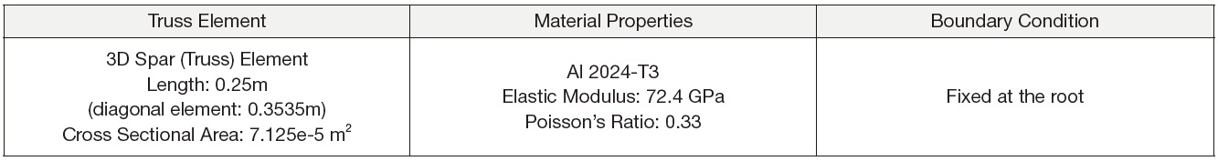
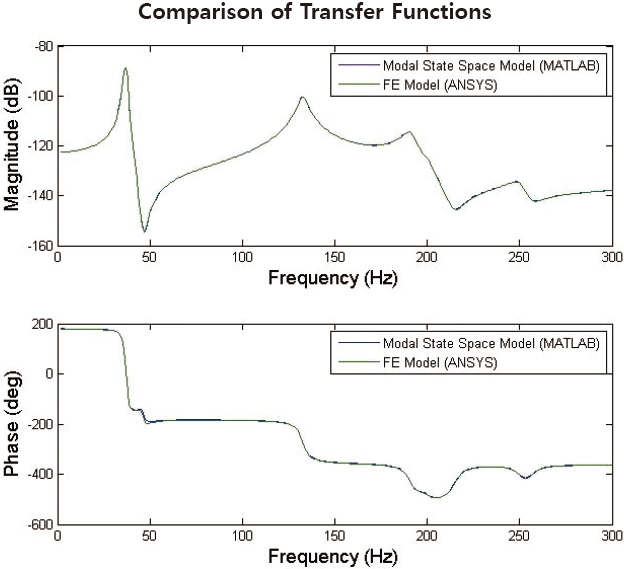
As this study is focused on the modeling methodology rather than on the accurate modeling of a specific structure, modeling a simple structure is preferable. So, a simple truss structure is selected. The structure is modeled in FE software by using the properties which are summarized in table 3, and the modal analysis is performed to derive the modal information. The obtained modal information is then used to create the state space modal model of the structure in MATLAB. By comparing the transfer functions of the model with that of FE model, the fidelity of state space modal model was checked. The results showed good agreement and they are as shown in Fig. 3.
[Table 3.] Properties of the truss structure.

Properties of the truss structure.
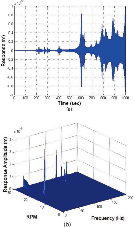
The obtained state space modal model is used to calculate the response of the truss structure to the reaction wheel induced disturbances. As the rotating speed of the reaction wheel is increased linearly from 0 to 30 Hz in 1000 seconds, the response of the truss structure (z-direction at node 18) to force disturbances Fx and Fy at node 9 is shown in Fig. 4 as an example. The waterfall plot shows a very large response when the second harmonic disturbance excites the first and the second mode of the truss structure. This occurs around 600 seconds when the rotating wheel speed is about 18 Hz, i.e. the second harmonic disturbance is about 36 Hz. Large response is also found when higher harmonics excite the structural mode of the reaction wheel at 150 Hz.
2.3 Cassegrain Reflector Modeling
In general, high performance optical payloads that are used in satellites are diffraction limited reflection telescopic systems. In this study, Cassegrain reflector which has a performance level of diffraction limited system is selected as the optical model. The effects of jitter that result in the performance degradation of the optical payload are expressed as a decrease in the value of module transfer function (MTF).
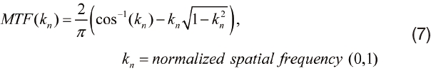
The MTF of diffraction limited system can be obtained by using the Fraunhofer diffraction equation for a circular aperture. The point spread function (PSF) of a system with an aperture that has a radius A at distance R can be obtained by squaring and normalizing the wave amplitude. The Fourier transform of the PSF is the MTF. The MTF of the diffraction limited system normalized by the cutoff frequency (kco) is given by using equation 7. The cutoff frequency is defined as kco = D/λf where, D is the diameter of the optical system, λ is the wavelength of the light and f is the distance to the focal plane.
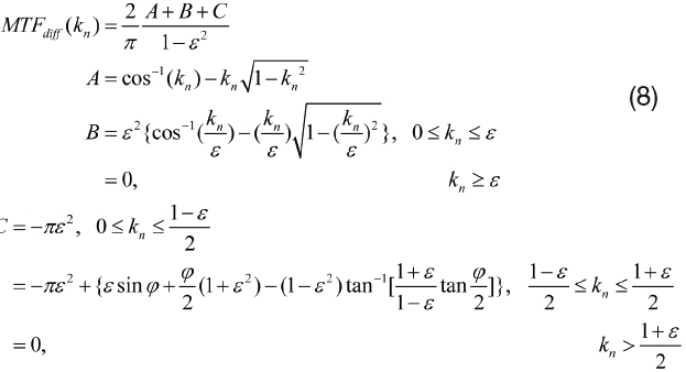
MTF for the effect of secondary mirror in Cassegrain reflector and it can be calculated by using the O’Neil’s formula [16] given in equation 8 where, ε is the ratio of the radius of secondary to primary mirror.
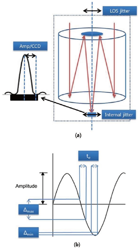
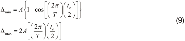
Depending on the movement of the optical structure and the frequency of the vibration disturbance, jitter effects can differ. Jitter effects due to the movement of the optical structure can be further divided into line of sight (LOS) jitter (movement of the structure as a whole) and jitter due to the relative motion of the optical structure which is as shown in Fig. 5 (a). The LOS jitter which is defined by using an angular displacement (θ) can be transformed to vibration amplitude at the focal plane through the multiplication of θ by the effective focal length of the optical system. Thus, jitter can be calculated by assuming the vibration of CCD focal plane. Jitter is also affected by the frequency of the vibration that is relative to the integration frequency of the camera (fe) and this is as shown in Fig. 5 (b). For the vibration frequencies that are lower than fe the amplitude of the vibration is phase dependent (equation 9), while for vibration frequencies which are higher than fe, peak to peak amplitude is used. In this study, only the worst case is considered by taking Δmax.
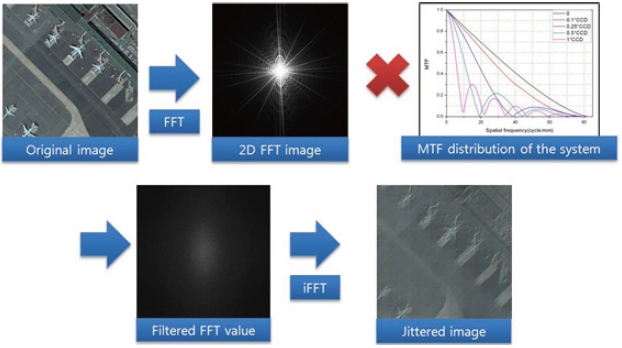
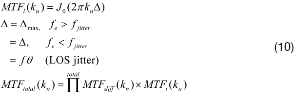
Considering the amplitude and the frequency of the vibrational disturbance, changes in MTF of the optical system can be calculated by using equation 10 [17]. The resultant MTF values can be used as a spatial filter at a focal plane for image simulation. For image simulation, FFT of the original image for R-G-B is obtained and the MTF of the jittered optical system is multiplied. Image that contains jitter effects can be obtained by multiplying FFT of a clean image by the MTF of the optical system and then, by performing back transformation. The procedure for image simulation using MTF value is summarized in Fig. 6.
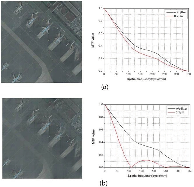
In this study, diffraction limited optical system that has sub-m resolution is used. The model is created by assigning ground sampling distance (GSD=1m), altitude of the optical system (h=685km) and CCD pixel size (7μm), by calculating the corresponding effective focal length ( f = CCDsize/GSD = 4.975m) and the radius of the optical system (a=1.22λf/ D=0.42m). Fig. 7 shows MTF of the optical model and image simulation results in the presence of 0.7μm (0.1 times the CCD size) and 3.5μm (0.5 times the CCD size) jitter.
2.4 Vibration Isolator Modeling
In the presence of excessive vibrational disturbances, LOS requirements for optical payloads may be violated. During such cases, active vibration control of structures [18] or implementation of vibration isolator is a feasible solution to limit the transmission of excessive vibration to sensitive optical payloads [19]. The most commonly used vibration isolators are the passive type and they are simple and reliable. For cases with demanding requirements that cannot be met by using passive isolators alone, active isolators can also be implemented for the enhancement of the performance but at the cost of increased complexity. Recently, hybrid isolators that comprise of passive and active isolators (SUITE [2], VISS [20], MVIS [21], and so on) have been developed to acquire the advantages and complement the disadvantages of passive and active vibration isolators.
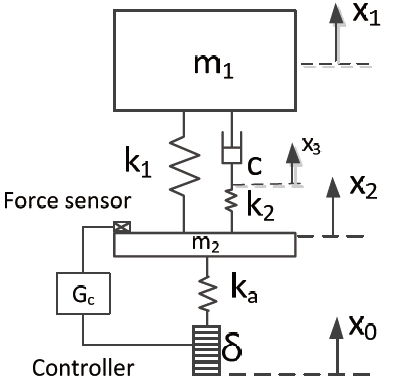
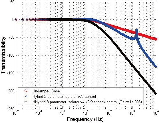
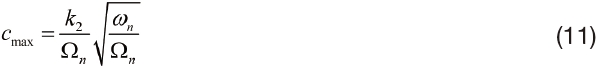
In this study, hybrid vibration isolator which is composed of three parameter passive isolator and piezoelectric stack actuator based active isolator that are shown in Fig. 8 are modeled. The three parameter isolator has an additional spring element (k2) in series with damper (c). By tuning the value of parameters k1, k2, and c, high damping at resonance can be achieved without sacrificing the high frequency isolation performance and this is a drawback with the conventional two parameter passive isolator. Maximum damping for the given values of k1 and k2 is achieved by using equation 11 where, ωn=(k1/m1) and Ωn=((k1 k2)/m1 [22]. Piezoelectric stack actuator, represented by its stiffness (ka) and extension (δ), is connected in parallel in order to enhance the performance of the vibration isolator.
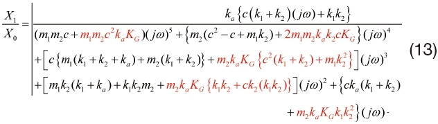
The value of the parameters m1, m2, k1, k2, c, ka used in this study are 5.9 kg, 0.118 kg, 23,000 N/m, 230,000 N/m, 610 Ns/m, 10,000,000 N/m respectively. For active control, force
at intermediate mass is measured and an integral controller is adapted. The control feedback signal and transmissibility of the isolator are given by the equations 12 and 13 respectively (the red colored terms in equation 13 indicates the terms that are due to active control). Fig. 9 shows the comparison of the transmissibility curves. For the same damping value the three parameter passive isolator shows much better isolation at high frequency compared to the conventional 2-parameter passive isolator, and the isolation performance can be further improved by using an active control.

2.5 Integrated Jitter Simulation Tool
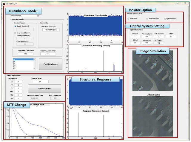
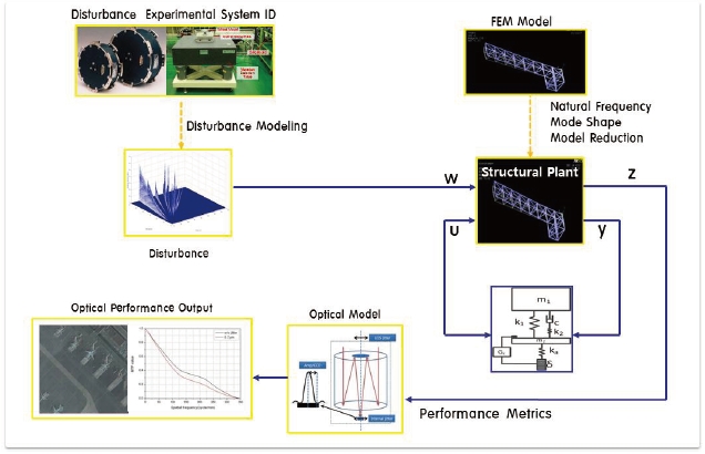
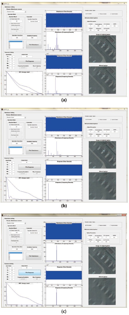
An integrated jitter analysis framework that combines disturbance, structure, optical system and vibration isolator model is developed by using MATLAB. The overview of the framework is shown in Fig. 10. Reaction wheel induced disturbance model can be generated by assigning parameter values that are based on the experimental data or reference values. The created disturbance model is then, used to provide excitations to the model of the structure in state space modal form which is derived by using the modal analysis results from finite element analysis. Based on the selection made by the user, vibration isolator can be used to isolate the generated disturbances. The response of the structure is calculated, and the result is used in the optical model to evaluate the performance degradation due to the induced vibrational disturbances. The interface of the simulation tool, shown in Fig. 11, is developed by using MATLAB GUI. Reaction wheel’s operational conditions, excitation input and response output nodes, isolator option, and optical model setting can be changed by using the user input. Plots of the disturbance and response of the structure in both the time and frequency domain, MTF of the optical system, and the image of the original and jittered system are displayed as the output.
By using the developed simulation tool, analysis on the performance degradation of the optical payload due to the reaction wheel induced vibration and the effectiveness of using vibration isolator in reducing the effects of jitter are done. Fig. 12 shows the simulation results to the disturbances in translational directions for reaction wheel operating speeds of 30 Hz, 37 Hz (natural frequency of the structure), and 150 Hz (natural frequency of the reaction wheel). The simulation results show that a considerable
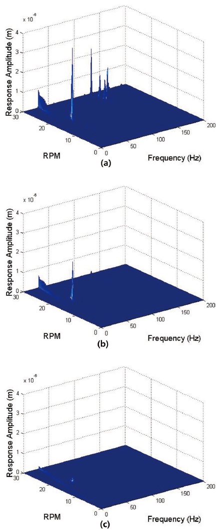
decrease in the optical performance is expected when the rotating wheel speed matches with the natural frequency of either the structure or the reaction wheel. Fig. 13 shows that the response of the truss structure to reaction wheel induced vibrations depending on the choice of vibration isolator that is used to isolate the generated disturbances. It can be seen from Fig. 13 that the structure’s response is much lower when a vibration isolator is used. Although the passive isolator eliminates most of the disturbances at high frequency, notable amount of disturbances remain in the low frequency range and this includes a significant peak around the first and second natural frequencies of the structure. Disturbances in the low frequency range can be further reduced by using a hybrid isolator and no significant peak is observed any more.
In this paper, an introduction to the development of an integrated simulation tool for the evaluation of the performance of optical payloads was given. The developed simulation tool comprises of the reaction wheel induced disturbance model, state space model of a structure in the modal form and the Cassegrain reflector model. The disturbances that were generated by using reaction wheel induced disturbance model are used to excite the structure modeled in the state space modal form. According to the user’s selection, vibration isolator can be used to isolate the generated disturbances, and the response of the structure is calculated. The result is used as a structural behavior input for the optical model for the evaluation of the performance
degradation due to the induced vibrational disturbances in terms of MTF and simulated image. Simulation results show considerable degradation in the performance of optical payload due to disturbances from the reaction wheel especially when the rotating speed of the wheel matches with the natural frequencies of either the structure or the reaction wheel model. Moreover, most of the jitter effects can be removed by using a vibration isolator. For future work, tests will be conducted for the experimental validation of the presented integrated jitter analysis framework.

![Analytical reaction wheel model with imbalance [13].](http://oak.go.kr/repository/journal/11310/HGJHC0_2012_v13n1_64_f001.jpg)