The Flower and Cook Observatory (FCO) of the Univer-sity of Pennsylvania (Penn) housed two main telescopes with professional research instruments. Attached to the 0.38 m (15 inch) Brashear-Fecker siderostat at FCO was a unique dual-channel stellar radiometer named the Pierce-Blitzstein photometer. A history of this instrument was already presented in Ambruster et al. (2011). For many years, attached to the FCO’s 0.72 m (28 inch) Fecker Cassegrain reflector was a series of elliptical polarimeters. Some history and descriptions of the polarimetric instru-mentation are already presented online in Blitzstein et al. (1993) and Koch (2010). The following report describes in detail the inception, development and extensive use over 30 years of elliptical polarimeters at Penn.

For decades, a worker on stars has easily recollected when photographic and photoelectric polarization pro-grams began on stellar targets. Polarization programs on general celestial targets may not be so easily in the mind of any specialist and the following is my personal recollec-tion of the first and futile polarization program at Penn.

In early 1955 I was notified that I would be awarded the Steward Fellowship at the University of Arizona starting in September. My recollection is that I had done essen-tially nothing to attain this award but I would have a lot of prospective use of the 0.9 m (36 inch) reflector which was functioning with a Newtonian photoelectric photometer and a double-slide photographic plate holder. F. B. Wood remarked only that I had essentially no observational ex-perience so far and I would have to accumulate that back-ground under the supervision of Leendert Binnendijk ef-ficiently.

I knew Binnendijk well from class work and was aware that he had had more than a little luck to survive World War II in Holland when his own early-mature resistance activity and then near starvation could have taken him off. I knew also that he had a varied background from astrometry and photometry and had accumulated a cer-tain number of variable star light curves. Largely through the effort of Peter van de Kamp, he had had four years at the Sproul Observatory and then had moved in 1951 to a faculty appointment at Carlton College, MN. At that loca-tion he decided to start moving away from his own photo-graphic experience toward photoelectric photometry and had a contract with the American Philosophical Society to support building just such a photometer. By the sec-ond year at Carlton, however, he had become aghast at the severity of the MN winters and was horrified that the school awarded an honorary degree to a man whose only attainment was to give money to the college. He wanted away from such an unscrupulous institution and he and Wood had a meeting that resulted in his arrival at Penn in 1953.

At this time there was no FCO but the staff had full-time use of the Roslyn House Observatory’s telescopes since G. W. Cook’s death in 1940. By re-negotiating his contract, Binnendijk’s new photometer would be installed on the

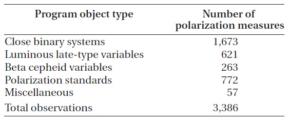
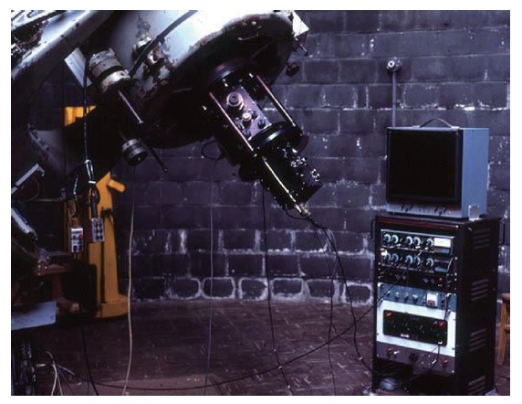
0.72 m reflector at the Cassegrain focus. Most of the ac-tual work to achieve this was done by William Blitzstein and his machinist from the Franklin Institute, Bud Thor-pe, and the reflector and photometer in their appearance until 1963 are shown in Fig. 1.

In very brief time Binnendijk was observing and his residence in Springfield Township made it easy for him to work several portions of nights per week. Wood and he talked about my situation and they agreed that I could pick up all experience I needed by working under Binnendijk’s supervision. This started on a frigid night?temperature was -9°C (15°F)？with Binnendijk observing some Pleiads, it moved to a second night when he ob-served a short-period variable, and continued night after night with me watching his activity at Cook. He had a rig-orous method of supervision: I should watch him as long as he worked on a night and I could watch the tape on the Brown Recorder, but I should never touch a single piece of hardware and I wasn’t encouraged to ask questions. This was not at all inspiriting but I felt I had no alternative but to come to Cook every night he observed. As spring moved along, one night something new happened. He twiddled a rotational control dial on the photometer that I had never noticed moved before and I had no alterna-tive but to ask explicitly what he was doing. He had direct-ed the telescope to 2 Pallas and wanted to see if it sent a polarized signal to Earth by him rotating an on-axis piece of Polaroid built into the photometer. No signal resulted. This experience didn’t help one’s beginnings at Steward.

Linear polarization signals from stellar sources observ-able at FCO tend to be small and on the order of a couple of percent or less of the flux. Natural stellar linear polar-ization arises from many sources including Rayleigh and Thompson scattering in the photospheres and circum-binary gas of program objects, Mie scattering by small silicate grains in the dusty atmospheres of late-type stars, and a linear polarization offset from the interstellar me-dium. Stars may produce significant circular polarization through magneto-opacity arising from Zeeman splitting in a thermal field, magneto-emission in stellar spots, and double scattering by birefringent grains in stellar atmo-spheres or interstellar medium. Many of the observable sources of elliptical polarization observable at FCO vary due to transients or by being phase-locked to a pulsa-tional or Keplerian period. Koch (2010) and Clark (2010) provide reviews of the relevant polarization literature and mechanisms.

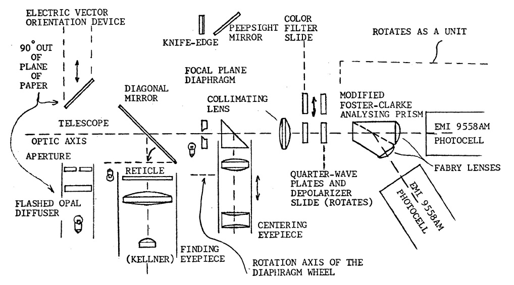
The first elliptical polarimeter at Penn, called the Mark I, began in 1967 as a term-paper design by George Wolf for William Blitzstein’s AST 504 Astronomical Instrumen-tation class. Blitzstein was interested enough in the paper to present the idea to the department chairman, Frank B. Wood, about the possibility of building the instrument. Wood offered Wolf the remaining funds in an expiring National Science Foundation grant to purchase all of the optics, and the optics were quickly purchased. The rest of the mechanical and electronic design was worked out by Blitzstein and Wolf. In 1968-69, department staff members William Barrie and Robert Smith worked on the machining and the electronics, respectively, to complete the instrument construction. Fig. 2 illustrates the optical configuration of the Mark I Polarimeter described by Wolf (1970, 1972).

For the main optical path, flux entered from the left and passed through a focal plane diaphragm, collimat-ing lens, filters mounted on a slide, oriented retarder plates mounted on a slide, Foster-Clark analyzing prism with attached Fabry lenses, and dual EMI 9558AM pho-tomultiplier photocells. The analyzer, Fabry lenses, and photomultipliers rotated as a unit through 360 degrees. Program object measures were made at eight orienta-tions 45 degrees apart and reduced to give the natural, unstandardized, Stokes I, Q, U, and V measures, and q, u, and v in percent. The two-channel integration data, filter

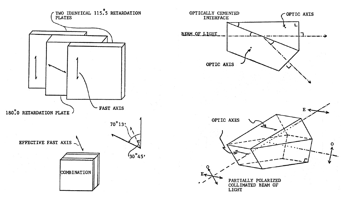
and position codes, and time for each measurement were recorded on punched paper-tape. Further details of the specialized optical components are illustrated in Fig. 3. Fig. 4 shows the completed Mark I polarimeter as it ex-isted in 1969.

The first use of the Mark I polarimeter was planned to be a southern sky elliptical-polarimetry survey by Wolf (1970, 1972) on the 0.61 m (24 inch) Optical Craftsman Telescope at Mt. John Observatory in New Zealand during 1969. However, because of design and mechanical prob-lems, that telescope was not delivered to New Zealand until 1970. This delay caused a change in venue to Kitt Peak National Observatory for a northern sky elliptical-polarimetry survey by Wolf during December 1969 and January 1970. Fig. 5 shows the polarimeter mounted to the 0.9 m on Kitt Peak. The polarimeter was then moved to FCO in 1971.

The initial elliptical-polarization survey (all four Stokes parameters) at Kitt Peak of approximately 70 objects included magnetic A stars, polarized O and B stars and highly polarized stars of other spectral types, stars with peculiar spectra, intrinsic variable stars, galactic and ex-tragalactic objects with known synchrotron radiation, comet Tago-Sato-Kosaka, and both unpolarized and po-larized standard stars. Many of the program objects were

previously known to be linearly polarized so the main val-ue of the Q and U Stokes measures were in the long-term monitoring for changes in the polarization signal. No sig-nificant V circular polarization parameter was detected for any of the program objects down at the 0.01% level.

A number of upgrades were made to the polarimeter over the decade of the 1970’s. Initially, the upgrades were designed to improve the efficiency and comfort of the ob-server. For instance, in 1972 a dual-channel HP integrat-ing digital voltmeter and digital clock were added along with a closed circuit TV camera which was trained on the on the digital displays of the clock and voltmeter. This up-grade meant that observers were able to sit in the heated control room rather than stand in the freezing dome in the middle of a cold winter night hand recording numeri-cal values. Additionally, between 1972-1973 an IBM key punch was interfaced with the digital voltmeter and clock so that the observer no longer had to key punch the hand written measures the next morning.

A major upgrade to the sensitivity operation of the po-

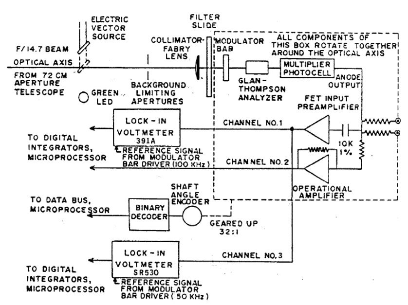
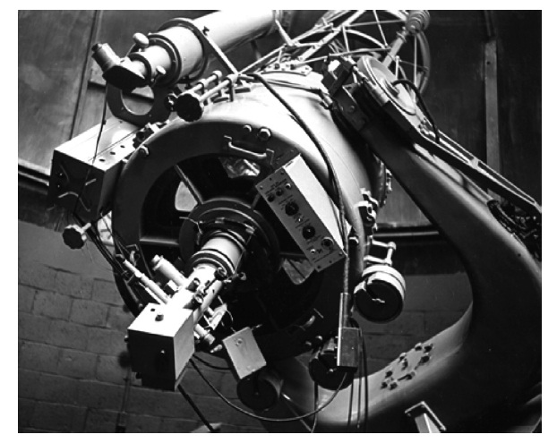
larimeter was accomplished over the period from 1977 to 1981. The polarimeter optical train was redesigned along the lines of a polarimeter built by Kemp (1969) to use a time-variable retarder instead of the statically ori-entated wave plates used in the Mark I instrument. Fig. 6 illustrates the electro-optical configuration of the newly named photoelastic modulating polarimeter (PEMP) as described in Elias (1990), Holenstein (1991), and Blitzs-tein et al. (1993). When measuring linear and circular po-larization the peak amplitude of the retardance was set, respectively, to one half and one quarter of the effective wavelength of the optical filter.

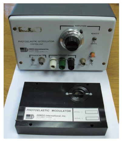
For the main optical path of the PEMP, flux enters from the left and passes through a focal plane diaphragm, col-limating lens, filters mounted on a slide, a photoelastic modulator bar of the type shown in Fig. 7, Glan-Thomp-son analyzing prism, and a single RCA 4509 photomulti-plier photocell. As in the Mark I instrument, the optical head rotated as a unit through 360 degrees. The output of the photomultiplier was amplified and fed into an Ithaco Model 391A analog lock-in amplifier operating at the reference frequency output of the PEM-3 (50 kHz) for the Channel 1 signal corresponding to the circular Stokes vector, or at twice the frequency (100 kHz) when measur-ing the linear Stokes vectors. The Channel 2 signal was integrated to give the average flux at each orientation of the optical head. Channel 3 will be described in a later section. According to Blitzstein, the Glan-Thompson ana-lyzer was chosen over the Foster-Clark unit because of its lower residual polarization induction and superior nu-merical aperture. Program object measures were made at nine or ten orientations of the optical head and reduced with a truncated Fourier least squares fit and instrumen-tal calibration factors to give the natural, unstandardized, Stokes q and u, or v measures in percent.

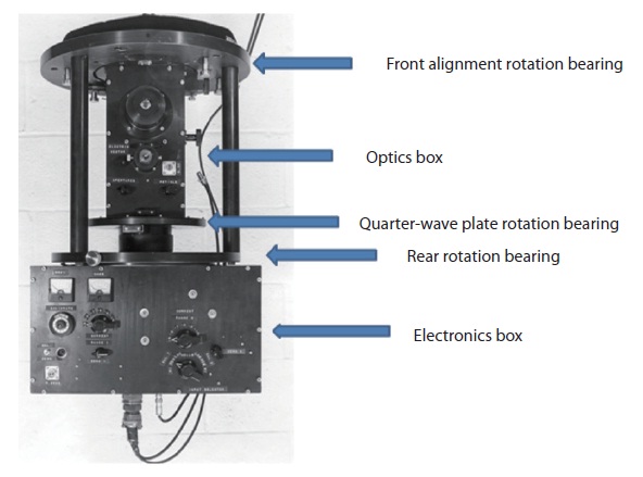
The late 70’s saw the introduction of several affordable microcomputer system brands suitable for scientific use. A lumber mill harvested a number of oak trees in the for-est surrounding the FCO and the funds were obtained to purchase two Ohio Scientific Incorporated microcom-puters in 1981, one of which was dedicated to the PEMP operations. Graduate student Dave Bradstreet wrote the first automated polarization data reduction program. Fig. 8 shows the PEMP and some control equipment as it looked when installed at FCO in the early 80’s. The first observations recorded in the log books were of an eclips-ing binary of the Algol type, HD 156247(U Oph) by Koch the night of August 17-18, 1981.

In 1982, an optical digital encoder was added to the PEMP in order to read accurately the orientation of the optical head. No longer was it a burden on the observer to accurately position the PEMP to designated orientations. The march of technological progress made the 8-bit CPUs of the Ohio Scientific computer obsolete and they were replaced with IBM AT microcomputers in 1986 and new digital integrator interface.

Bruce Holenstein’s employer acquired a Stanford SR530 lock-in amplifier for a solar scintillation study he was conducting with Blitzstein at FCO and Kitt Peak. After those experiments concluded with mixed results, Holen-stein added the Stanford lock-in to the PEMP in 1986 and wrote the computer program to comprise the Channel 3 illustrated in Fig. 6 thereby doubling the productivity of making elliptical polarization measures with the PEMP. Channel 3 was dedicated to operating at the PEM-3 refer-ence frequency so it was sensitive to the circular Stokes parameter. In order to preserve five years of linear polar-ization standardization data already taken with the PEMP, a decision was made by Blitzstein, Koch, and Holenstein to run the new elliptical polarimeter configuration with the PEM-3 set to the peak retardance for making linear polarization measures with Channel 1. This setting result-ed in a 30% reduction in sensitivity of Channel 3.

Some of the electrical components of the PEMP, such as the voltage controlled oscillators, were found to be temperature sensitive. In 1987, temperature sensors were installed into the PEMP and the Channel 1 Ithaco lock-in amplifier. The reduction software was modified to factor the temperature data automatically into the natural mea-surement values.

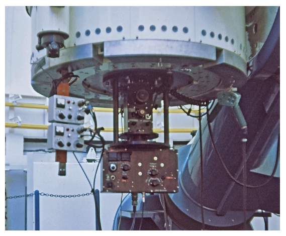
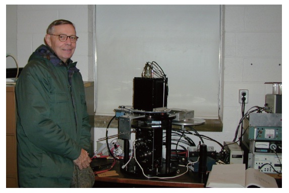
The last major polarimeter upgrades were completed between the late 1990's and 2000 in anticipation of a move of the PEMP by Nicholas Elias to an observatory which did not allow observers in the dome while obser-vations were underway. So, remote operation control was completed for the filter slide and orientating the optical head. Fig. 9 shows the final PEMP device.

For several years there was only concern about the change in the Stokes linear parameters either with time or phase-locked to a Keplerian ephemeris for a program object. This really meant that there was little interest in whether the natural system measured by the polarimeter changed as the instrument was taken off the reflector and then re-installed or was retained on it for a lengthy time. Over a few years the polarimeter was commonly removed monthly because the double-slide plateholder was given dark-of-the-moon time and the polarimeter shared the other half of the lunar cycle with an IR detector. It was also removed in order that the telescope optics could be cleaned with some frequency.

Eventually, this minimal attention was recognized to be a significant instrumental problem since non-normal, or at least non-axisymmetric, reflection or transmission off of or through an optical surface or non-uniform coat-ing would induce a potentially significant polarization offset and change of instrumental gain. As a result, an extended effort was committed to a literature search that would identify fairly bright, northern stars that had been observed repeatedly and, if possible, by more than one group. Many of our final identifications of null standards emerged from the very early individual workers such as Hall & Mikesell (1950), Hiltner (1956), and Behr (1959); only sample references are indicated here. The FCO tele-scope log lists the first null standard to be HD 188512 (β Aql) in August 1972 and the summary by Koch & Clarke (2005) notes that 929 linear and 335 circular Stokes pa-rameters were accumulated for 35 and 12 null standards, respectively, over 25 years by numerous observers. (Only 2 measures were accidentally omitted from this list.) There was some suspicion that HD 61421(α CMa) and HD 172167(α Lyr) did not have constant circular components but all the rest of the measures were certainly not variable in any Stokes parameter.

Even though for the program’s beginning there had been observed a few stars that were known or believed to be polarized constantly, this was a minor effort because most of the program stars were themselves of very small polarization. Eventually this changed and there were begun to be observed in 1977 a certain number of stars believed to be considerably and constantly polarized by interstellar dust. Beginning in 1977, non-null standards were mostly taken from surveys at Arizona (Coyne & Kruszewski 1969) and they permitted observing consid-erably polarized program stars. The summary of this ef-fort appears in Koch (2006) although with rather small emphasis therein to the work itself. For instance, 202 linear measures were observed of 19 stars and 38 circular measures of 11 such standards, one of which reached p as large as 6%. (By accident, five measures were acciden-tally omitted from Koch’s reporting of these results but this omission also had no effect.) This suggests that one should be able to standardize essentially all program stars confidently but the potential problem with this interpre-tation is that eight of these non-null standards had been identified in 2006 as light variables. Koch’s paper called attention to this circumstance with the possibility that these standards could themselves be polarization vari-ables leading to erroneous calibrating of program stars.

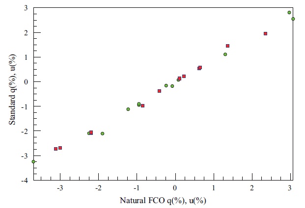
Lists were compiled so as to work on standardizing candidates for repeated FCO observing as frequently as possible through all four filters. Since a single colored measurement required about 30 minutes of time, this definitely took time away from the program stars. The sci-entific return from the effort was to be able to say that the instrument was in a fixed condition during the observing program and that the local measures could be turned into a standard set of measures. A sample set of data appears in Fig. 10 representing the green standard measures from November 1982 through May 1983 after the optics had been re-aluminized.

It is obvious that one can make linear least-squares calibrations turning the natural measures into standard ones. For this particular example:

The standard deviations of these coefficients (which follow the numbers) are quite constant over the entire program once the standardization started; this may be verified by the example results for the following year pub-lished by Koch & Clarke (2005).

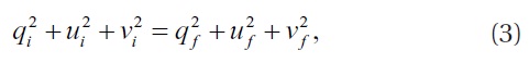
The standardization of the circular Stokes parameter was better than the precision just quoted for the linear parameters because most of the standards had essentially zero values and not large positive or negative values. In order to standardize and check the magnitude of the cir-cular parameter, a hybrid method of standardization was chosen to piggyback on the standardization of the linear parameters. A quarter wave plate retarder was inserted into the optical train ahead of the photoelastic modulator in order to introduce a rotation on the Poincare Sphere and convert some of the known linear polarization from

a linear polarization standard star or electric vector linear polarization calibration source into circular polarization. The invariance relation for the rotation is given as follows:

where the subscripts i and f refer, respectively, to the po-larimetric values prior to and after the insertion of the quarter wave plate. In accordance with a resolution of International Astronomical Union Colloquium 23, the convention for positive circular polarization was adopted to be a counter-clockwise rotation of the electric vector when the detector faces the program object. For the pe-riod 1987-1990, the circular polarization standardization in the V-bandpass was calculated to be:

A continual search for non-null circular polarization standards with apparent magnitudes observable at FCO remained a focus throughout the history of the observ-ing programs. In addition, precision laboratory circular polarizing films and sources were constantly obtained whenever available but were only found to be sufficient to check the standardization as they were not found to have a better accuracy over the hybrid circular polariza-tion standardization method utilized at FCO. The ellipti-cal standardizing programs continued until the end of the FCO.

Blitzstein et al. (1993) reviewed the FCO observing logs and tallied the observing statistics as presented in Table 1. Each program object measure represented about 25 to 30 minutes of time observing at the telescope. Typically, this was because nine or ten orientations of the PEMP were used, and at each orientation, the program object and background were observed usually for a total of two minutes. The remaining five to ten minutes of overhead time was consumed in software inputs, filter selection, rotating the PEMP optical head, and slewing to the back-

ground and centering the program object at each PEMP orientation.

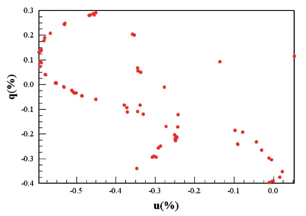
Koch (2010) chronicles in some detail the contribu-tions to astronomy made by polarimetric observers at Penn. In addition to the survey by Wolf (1970, 1972), the observations programs accomplished with the successive generations of Penn polarimeters included PhD theses by Pfeiffer (1975) on eclipsing and spectroscopic binary stars such as HD 1337 (AO Cas); Bradstreet (1983) on the K-type overcontact binaries CC Com, FG Sct, BI Vul, FS CrA, and VZ Psc; Corcoran (1988) on the massive close binary HD 215835 (DH Cep); Elias (1990) on eclipsing “serpentid” bi-naries HD 232121 (SX Cas) and HD 198287 (V367 Cyg); and Holenstein (1991) on the luminous late-type variables HD 36389 (119 CE Tau), HD 39801 (α Ori), HD 42543 (6 BU Gem), HD 44537 (Ψ¹ Aur), HD 97778 (72 Leo), HD 115898 (V CVn), HD 148478 (α Sco), HD 156014 (α¹ Her), HD 206936 (μ Cep), HD 208816 (VV Cep), HD 217906 (β Peg). Some data from Holenstein’s thesis is plotted in Fig. 11. Elias et al. (2008) summarizes and interprets previous-ly unpublished data for numerous program stars.

By 1993, the approximately 40 acres of land surround-ing the FCO had appreciated enough in monetary value

to be an attractive source of potential revenue for Penn. Overtures to sell the FCO property through a local devel-oper resulted in the sale of the surrounding 36 wooded acres with an island of only four acres remaining to pro-tect the FCO from neighbors’ lights. Upon Koch’s retire-ment in 1996, the PEMP system was no longer used regu-larly and so Elias and Koch planned a move after the final system upgrades in 2000 to Flagstaff, AZ and temporarily mounted the device on the United States Naval Observa-tory 1.0 m (40 inch) reflector. No scientific measures were recorded with the PEMP at its last mounting location.

Elias has preserved the final PEMP device and has it in storage in New Mexico awaiting a suitable telescope and observer availability. Holenstein has preserved at his of-fices in Malvern, PA the FCO observing logs and Blitzs-tein’s and Koch’s files on the various Penn polarimeters.

Polarimeters at Penn evolved over 30 years and uti-lized the best available technology during that time to both improve efficiency and sensitivity. The instrumental improvement and scientific programs conducted were a product of a collaboration of many Penn astronomers and staff from 1967 to 2000. Elliptical polarimetry, using a photoelastic modulated bar, was a productive activity at FCO, a location with considerable light-pollution from a major US city. Objects all over the HR diagram down to about 11th magnitude were successfully studied po-larimetrically. The precision in later years of better than +/-0.01% for a 7th magnitude star was routinely accom-plished for the Stokes q and v vectors.