The collision risk of space objects with satellites in operation is currently getting higher with the increasing number of space objects. Accordingly, satellite operating agencies need accurate space situational awareness (SSA) of satellites and space objects. SSA uses the position and velocity information of earth-orbit objects obtained by optical telescopes and radars, which further includes sizes of space objects, shapes of satellites, performances of payloads, intelligence, reconnaissance, etc. in military areas.
Individual satellite operating agencies in each country have been monitoring space objects and satellites in operation, and the Korea Aerospace Research Institute (KARI) is performing a preliminary analysis on conjunction and SSA for their satellites in operation (Jung et al. 2012). The most typical data for SSA is the two line element (TLE) provided by the Joint Space Operations Center of the United States Strategic Command (USSTRATCOM). The Joint Space Operations Center generates orbital information by tracking space objects and publishes mean orbital elements of approximately 16,000 space objects in the format of TLE (NASA Orbital Debris Program Office). Most satellite operating agencies and countries use self-generated data and TLE data in parallel for their SSA. Accuracy of results from using TLE is affected by various types of uncertainties such as uncertainty by the simplified general perturbation 4 (SGP4) model, which is widely used for orbit predictions, uncertainty in orbit propagation by the atmospheric parameter, and uncertainty by the accuracy of tracking and orbit determination. Although TLE data are widely used in public, any preliminary analysis of initial conjunction is not possible without knowing the precision of the TLE data. Estimation methods for the uncertainty of TLE data have
Space objects.
been mentioned in a number of papers, but the validity of those methods and TLE precision are not fully understood. Therefore, we analyze precision of the Korea Multi-Purpose Satellite-2 (KOMPSAT-2) TLE and validate those TLE data with the true orbit.
The first purpose of this paper is to determine the precision of TLE data and estimate a covariance matrix through an analysis on residual variation of TLE state vectors using TLE data available in public. The TLE data of KOMPSAT-2 distributed over 15 days are propagated using SGP4 from the each TLE epoch to the reference TLE epoch. Residual variation characteristics and covariance matrix representing positional uncertainty can easily be understood from differences in position and velocity between the TLE state vector and each propagated state vector at the identical epoch. As a satellite has unique characteristics depending on the orbit in general, the characteristics of the residual variation of the state vector and covariance may have common elements for all satellites and specific elements only related to that satellite (Osweiler 2006). In this paper, we analyze the characteristics of TLE by estimating covariance and variation of the radial, in-track, and cross-track components of the TLE of KOMPSAT-2.
The second purpose of this paper is to examine and analyze the validity of the above method developed and used for the first purpose. We use independent orbit data with an accurate precision for this validation. Confidence in the results from the first method can be secured by comparing the position residuals and covariance derived from data with an accurate orbit precision to those only from TLE. If the state vectors from the true orbit data are consistent with the state vectors from the TLE data in the estimation of position residuals and covariance, this implies that the method used for the first purpose is appropriate.
This chapter covers the methodology by which the position residuals of TLE is analyzed and the covariance is estimated. Prior to achieving the primary objectives, preliminary work is required, including selecting the space objects and gathering TLE data. Next, coordinate system and transformations are defined. The method by which the TLEs are propagated accompanied with an explanation of data binning. Finally, the estimations of the covariance matrix at the identical epoch for each space objects are discussed.
2.1.1 Selection of Space Objects
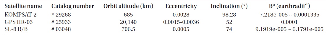
The first step in the analysis of residual variation of the state vector and covariance is to select the space objects to be analyzed. Among the numerous space objects in the earth orbit, we select satellites with true reference orbits available. Next, medium earth orbit (MEO) and low earth orbit (LEO) satellites are selected for an analysis on intrinsic characteristics depending on altitudes. Also, we select one of the space debris with a high possibility of approaching to KOMPSAT-2 which was known by a previous analysis of conjunction. Table 1 presents characteristics of the selected space objects arranged with the TLE data. Here the period of analysis is the time range within which true orbit data are available and the altitude is the mean altitude.
2.1.2 Space Object-Based Coordinate System
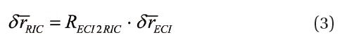
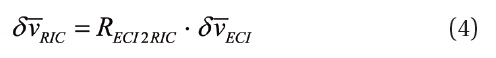
A space object-based coordinate system has an advantage over the earth-centered coordinate system in investigating the relative motion of the space object and any influence by the atmosphere. The radial, in-track, cross-track (RIC) coordinate system is one of the space object-based coordinate systems. In this paper, the R-axis represents the radius vector where a position vector propagated to the identical epoch is pointing to the position vector at the TLE epoch, and the C-axis is derived from the outer product of the radius vector and the vector in the direction of motion. Lastly, the I-axis is from the outer product of the vectors of the C-axis and the R-axis. Hence, the position and velocity vectors in the earth-centered coordinate system are transferred to the RIC coordinate system. The RIC coordinate system is often used for describing orbital errors, relative positions, and orbit changes of space objects.
2.1.3 Orbit Propagation
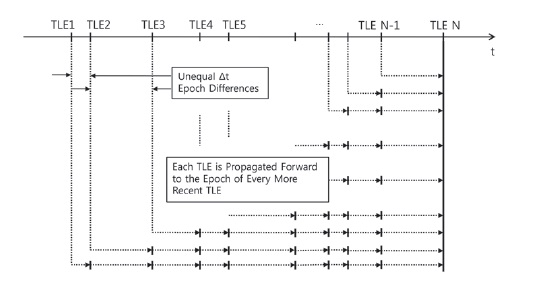
We use the pair wise differencing method (Osweiler 2006) to analyze the position residual and covariance between different TLE data which are used for the orbit propagation. As a comparison between the position residuals or the covariances existing within the TLE data is only possible at the identical epoch, the TLE data are required to be propagated to the same epoch of comparison. The primary reference epoch is set by the N-th epoch which is the epoch of the most recent data among the existing TLEs in the given range of time. At this point, the position and velocity vectors of TLE are most reliable and the TLE is the published TLE without any propagation. Position and velocity vectors propagated from the N-1-th epoch of TLE to the N-th epoch are derived. Then, the state vector propagated from the N-1-th epoch to the N-th epoch is subtracted by the state vector at the N-th epoch, which is called residual. This process is described by Eqs. (1) and (2). Now the state vector propagated from the N-2-th epoch to the N-th epoch is subtracted by the state vector at the N-th epoch. This process is repeated until the state vector propagated from the first TLE epoch to the N-th epoch is subtracted by the state vector at the N-th epoch. In the next step, setting the N-1-th epoch as a new reference epoch, a residual is calculated with the state vector propagated from the N-2-th epoch. Again, a residual is calculated for the state vector propagated from the N-3-th epoch, and this is repeated until the residual with the state vector propagated from the epoch of the first TLE is calculated.
Such a process is repeated on to derive the residual of the state vector propagated from the first TLE epoch, with the second TLE as the reference. Fig. 1 describes this statistical analysis, which is called the pair-wise differencing propagation.
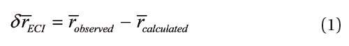
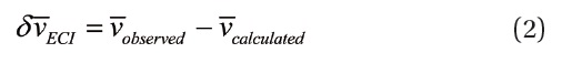
As the calculated residuals of position and velocity are defined in the earth-centered inertial coordinate system,
those values are transferred to the RIC coordinates, where the space object is the reference, to derive relative differences. Eqs. (3) and (4) are used for the transformation to the RIC coordinate system.
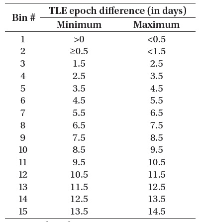
2.1.4 Data Classification into Time Blocks
In general, TLE data are provided at unequal time intervals. Thus the epoch time difference in between TLE data, Δ
The time blocks should be set appropriately in balance between the errors of observational data and the number of data arranged to each block, and the results of statistics are affected by the size of blocks. One-day interval is rational for an initial study and selected to keep the computing time throughout the process. A larger time interval provides better statistics but a poor figure for distribution.
2.1.5 Residual Variation
By analyzing the residual variation derived by using the TLE data, accuracy and variability of the propagated TLE
[Table 2.] Delta epoch bin ranges for 15 bins (Osweiler 2006).

Delta epoch bin ranges for 15 bins (Osweiler 2006).
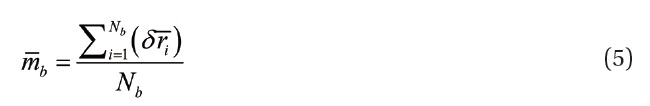
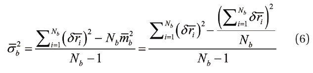
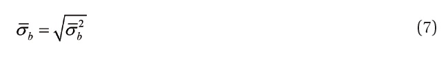
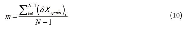
data to different epochs can be examined. The analysis of residual variation is achieved by analyzing mean, variance, and standard deviation of the propagated TLE data to different time blocks. The mean, variance, and standard deviation are calculated by Eqs. (5-7). Here δ

denotes the position residual, Nb is the number of components in each time block, b represents the time blocks (b = 1, 2, ..., 5), and

are mean, variance, and standard deviation in each time block, respectively.
2.1.6 Estimation of Covariance Matrix
The covariance matrix can be estimated using the residual derived from the differences between the N-th state vector and the other state vectors propagated from individual TLE epochs, except for the N-th TLE, to the N-th epoch(Osweiler 2006). The calculated state vector of the N-th TLE,

is regarded as the best state vector since the true value at the N-th epoch is not known.

is the propagated TLE state vector from each epoch to the N-th epoch, and δ

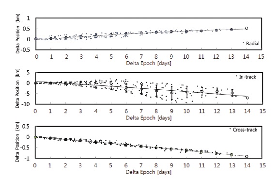
We propagate TLE data published from September 12, 2011 to September 26, 2011 for the accuracy analysis of the KOMPSAT-2 TLE. The TLE data are available from space-track.org and the total number of the TLE data within this period is 50. The orbit propagation is performed by the
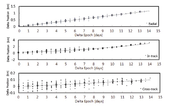
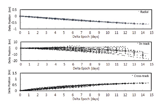
SGP4 propagator in satellite tool kit (STKⓡ) and the RIC components are derived by the report function (Analytical Graphics Inc.). Fig. 2 shows the residual variation of the state vectors of KOMPSAT-2. The horizontal axis is for the propagation time in 15 time blocks at a constant interval and the vertical axis is for the residuals of three components of radial, in-track, and cross-track in the RIC coordinate system. Mean and standard deviation within each time block are calculated by Eqs. (5-7) as presented in the figure. The standard deviations are expressed as the vertical error bars extended in both directions from the mean values. The mean and standard deviation reflect the accuracy and variability of the state vector residual in each time block, respectively. The dotted line in Fig. 2 is added as a fitting line by the least-square method of second-order polynomial.
The residuals of state vector are distributed in the form of a curve, which is determined by the characteristics of the SGP4 dynamics model used in the analysis. The error in the in-track direction is relatively larger than those in the radial and cross-track directions, which implies that the in-track component is highly affected by the perturbation component by the atmosphere. Also, the errors in the radial and cross-track directions appear stable regardless of time blocks.
Averages of the individual RIC components over the time blocks of 15 days are approximately 0.60 km, -11.00 km, and 0.64 km, respectively, and the RIC averages for one (1.027) day propagation are stable with approximately -0.057 km, 0.052 km, and 0.072 km, respectively. Such characteristics of the TLE state vectors of KOMPSAT-2 are planned to be reflected to the actual, initial operation and used for the SSA of space objects.
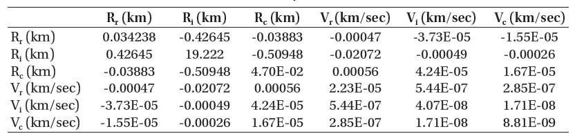
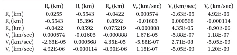
The covariance matrix of KOMPSAT-2 can be derived from the firstly obtained residuals of the RIC components of TLE. In the calculation of covariance matrix only using the TLE data, as the actual state vector cannot be known, we regard
[Table 3.] Covariance matrix of KOMPSAT-2 (only TLEs).

Covariance matrix of KOMPSAT-2 (only TLEs).
[Table 4.] Covariance matrix of GPS IIR-03.

Covariance matrix of GPS IIR-03.
the 50-th TLE data, the latest one, as the best prediction of state vector to calculate the covariance from the residuals in the RIC directions at the identical epoch. Table 3 presents the covariance matrix calculated by the TLE data of KOMPSAT-2. The diagonal terms of the matrix represent the variances of 6 state components, respectively, and the off-diagonal terms are the cross-correlations between different state components. The in-track component of state vector is the largest value in the covariance matrix and represents the worst uncertainty related to the estimation of state vector.
In the case of global positioning system (GPS) IIR-3, the number of published TLE data over 2 weeks of the same period is 20 and the orbit propagation is performed by the SGP4 propagator. Three components expressed in the RIC coordinate system are distributed to the time blocks at an interval of one day and plotted as shown in Fig. 3, together with mean, standard deviation and a least-square curve in each time block. The residuals in the in-track direction are not so large as those of KOMPSAT-2. This is because of the more stability without a dominant perturbation at the
satellite altitude of about 20,000 km which is classified as MEO. Also in Table 4, it is confirmed that the variance of the positional component in the in-track direction, 0.608 km, is smaller than that of an LEO satellite which is highly affected by a perturbation.
Similarly, in the case of SL-8 R/B, variations of the RIC components are derived from 27 TLE data published during the same period through the SGP4 propagator. It is shown in Fig. 4 that the residuals in the in-track direction component are influenced by the perturbation by the atmosphere. The RIC averages for one (1.029) day propagation are approximately 0.033 km, 0.062 km, and -0.053 km, respectively. Table 5 is for the covariance where the variance of the in-track component is about 15.40 km.
The in-track results of residual variation over about 1 day in LEO are approximately 0.052 km for KOMPSAT-2 and 0.062 km for SL-8 R/B, respectively. The range of those results is consistent with other studies in the past (Kim et al. 2010b).
[Table 5.] Covariance matrix of SL-8 R/B.

Covariance matrix of SL-8 R/B.
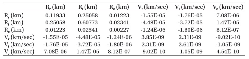
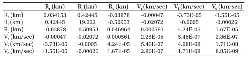
[Table 6.] Covarianc matirix of KOMPSAT-2 (with truth data).

Covarianc matirix of KOMPSAT-2 (with truth data).
The analysis of residual variation of the state vector and covariance in Section 2 is performed by using TLE data. The validity of such an analysis needs to be verified by another, separate method. Variations and covariances can be examined and compared between the actual state vectors of the satellite and its TLE data. A satellite operating agency can apply such a verification method to the satellites in actual operation to derive meaningful results representing propagation characteristics in the individual orbits.
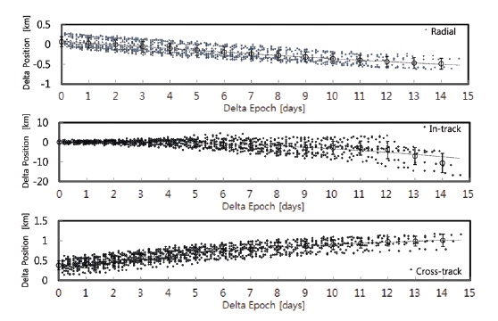
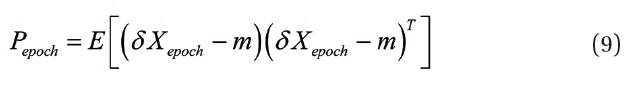
We validate the methods of state vector variation and covariance matrix estimation for KOMPSAT-2 which is in operation by KARI. In the analysis of state vector variation where the residuals are calculated at each epoch of the TLE data, the actual data of state vectors of the satellite should be fitted into the epochs of the TLE data (Mason 2009). In the case of KOMPSAT-2, the actual position, which is reported every 30 seconds, is propagated by the high precision orbit propagator (HPOP) from the closest point before the corresponding TLE epoch to the TLE epoch. The RIC residuals are calculated between the state vectors from the TLE data and those from the actual data. Mean, variance, and standard deviation of the residuals are calculated by Eqs. (5-7) and the covariance matrix is derived by Eq. (9).
In the case of KOMPSAT-2, orbital information at a precision level of 3 m can be obtained by determining the orbit through the internal HPOP using GPS navigation solutions (Kim et al. 2010a). The position reported every 30
seconds is regarded as the best state vector of KOMPSAT-2. In the estimation of state vector variation, the residuals are calculated at the epochs of the TLE data of KOMPSAT-2. Thus, to obtain a true orbit state vector at the same epoch as that of TLE, the former state vector (30 seconds, 00 second) close to the TLE epoch is propagated to the TLE epoch by the HPOP in STK and the perturbation model used in the real HPOP. Accordingly, the residuals in each direction at the identical epochs are compared to estimate the position residual and covariance matrix, which are presented in Fig. 5 and Table 6, respectively. Fig. 5 is the plot of state vector variation derived from the precise determination of the true orbit, which shows the identical characteristics in all the three directions of RIC with the state vector variation only from the TLE data (Fig. 2). When comparing the mean values and standard deviations of the residuals in each time block, however, the mean and standard deviation of the residuals derived from the true precise orbit are larger than those from the TLE data. The larger deviations compared to the deviation components of the TLE data (Fig. 2), which are for the mean orbit, can be explained by that the true orbit
[Fig. 5.] RIC residual variation of KOMPSAT-2 (with truth data). RIC: radial, in-track, cross-track.

is an osculating orbit which has larger deviations in the residual components as seen in Fig. 5.
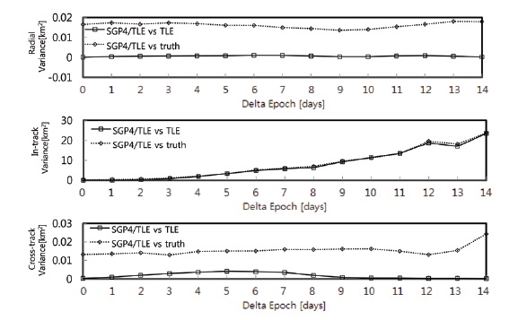
For a clear comparison, Fig. 6 shows the variance of residuals only from the TLE data and that from the true orbital data. In the comparison of the variances in three directions, the variances calculated from the actual values of precise orbit determination are always higher than those from the TLE data. This coincides with the comparisons for the results of mean and standard deviation. Also, the degree of covariance is highly consistent with each other in the comparison of the covariance matrices from the TLE and from the true orbit determination (Tables 3 and 6). This validates the estimation of a covariance matrix through TLE, which can be used to calculate the probability of existence in which part in the space.
This paper describes the methods of analyzing the characteristics of residual variation and estimating a covariance matrix only using TLE data. Those methods were validated by using the true orbital data of KOMPSAT-2.
Residuals in the RIC components of three directions were calculated by using the TLE data and the SGP4 propagator, and it was confirmed by mean and standard deviation of the residuals depending on the time blocks that the satellite is disturbed by perturbation. Also, a covariance matrix representing uncertainties in the TLE state vectors was calculated.
In the case of KOMPSAT-2 classified as an LEO satellite, the in-track components of the residual variation and the covariance matrix values were the largest compared with those in the other two directions, which is evidence of a large effect by the atmosphere.
According to the plot for residual variation, this means that the TLE prediction using SGP4 becomes worse with increasing propagation time. The TLE estimation method described in this paper was validated by comparing and analyzing the results of residual variation and covariance matrix estimation from the true orbit with those from TLE. Also, the uncertainties inherent in TLE were analyzed through this validation and it was confirmed that the TLE data of KOMPSAT-2, published 3-4 times a day, were reliable as preliminary data for the analysis of initial conjunction.