Multibeam sonar systems are relatively new instruments compared to sounders; they have broad coverage and produce high resolution data samples. Hence, these systems have been increasingly employed to elucidate the ecology and population of aquatic organisms. A type of multibeam sonar (i.e., an imaging sonar), also known as the dual-frequency identification sonar (DIDSON) and sometimes an acoustic camera, has been widely used among fisheries acoustic scientists. It was created and produced by Sound Metrics (Lake Forest Park, WA, USA) and developed originally for the US Navy by the University of Washington’s Applied Physics Laboratory. DIDSON was initially used for structural inspections, leak and flow detection, underwater surveillance, and other underwater applications. Its applications have been adapted to fisheries, bridging the gap between existing sonars for fisheries resources estimation and optical systems (Moursund et al., 2003). DIDSON has two frequency modes, which allow flexibility in resolution and range. Using the high-frequency mode at 1.8 MHz greatly enhances image quality because the image is formed using 96 beams, each 0.3^° wide. The low-frequency 1.1 MHz mode consists of 48 0.6^° beams. The detection range of the higher frequency is available up to 12 m, whereas that of the lower frequency is approximately 30 m (Mueller et al., 2006). DIDSON records video-quality data and thus requires a great amount of disk space.

DIDSON applications can be largely categorized into fish counting, sizing, and the study of fish behavior, based on the research aim. Fish counting has been applied not only to salmon but also to jellyfish, steelhead trout, and small-sized fish (Holmes et al., 2006; Burwen et al., 2007; Han and Uye, 2009; Pipal et al., 2010). Salmon size in particular has been an application strongly demanded by scientists and anglers. Fish behavior in diverse environments (e.g., fish gears, redds, fishways, and locks) has been observed for ecological studies (Tiffan et al., 2004; Rose et al., 2005; Baumgartner et al., 2006). Accordingly, the main purpose of DIDSON would be defined as being to study fish counting, fish sizing, and fish behavior. Therefore, analysis software for DIDSON data should be capable of enumerating and sizing fish and investigating fish behavior. However, the volume of recorded data is huge; often approximately 1.8 gigabytes per hour is collected, so data processing power must be considered. Herein, sophisticated analysis software was required to handle and process the vast amount of data at high speed. In fact, recent advances in computer hardware and software have allowed faster, more efficient data analysis techniques.

The fisheries acoustic data analysis software Echoview (Myriax Pty Ltd, Hobart, TAS, Australia) is an application for DIDSON data and has been used among diverse groups of aquatic acoustic scientists for various objectives such as fish stock assessment, ecological monitoring, and environmental management. The capability of Echoview to handle DIDSON data analysis is recognized among many DIDSON users. However, the entire and precise process of DIDSON data analysis in Echoview may not be well understood. Echoview provides an environment, called the variables and geometry window, to create data flow. Yet, making a multifunctional data flow using DIDSON data to achieve the primary objectives mentioned above may be complex.

Recently, two studies were published concerning an automated analysis of DIDSON data (Handegard and Williams, 2008; Han et al., 2009). One study focused primarily on fish behavior, and the other was designed for fish counting and sizing. However, so far, these analysis methods have not covered the comprehensive aims of DIDSON applications. Therefore, an objective of this study was to evaluate the utility of a semiautomated analysis method using DIDSON data in Echoview for fish counting, sizing, and fish behavioral studies. A semiautomated analysis of the DIDSON data using Echoview was precisely evaluated using testing data sets collected on the Rakaia River, New Zealand. The process of semiautomated analysis is described step by step to yield fish counts and to extract the characteristics of fish biology and behavior, such as length, thickness, changes in depth, and speed.

Data were collected at Hydra Waters, a tributary of the Rakaia River near Christchurch, New Zealand. Migrating quinnat salmon Oncorhynchus tshawytscha were targeted. The DIDSON system was deployed in a fixed location (43^°15′41˝S, 171^°20′37˝E). Data were collected from 00:00:38 on May 11, 2009, to 23:51:33 on the same day. The DIDSON system is a type of sonar, consisting of multiple pings, which are also called frames in some studies (Moursund et al., 2003; Burwen et al., 2007; Mueller et al., 2010). The total number of beams per ping was 48, and the angle of the beams was between -14.13^° and 14.13^°. The maximum depth of data collection was approximately 20.4 m.

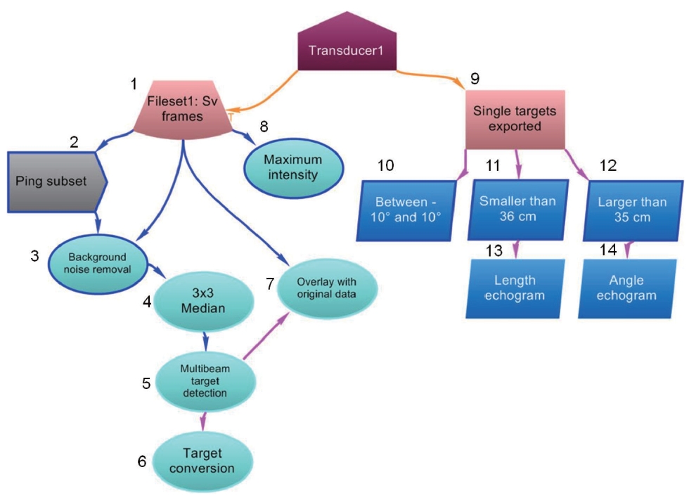
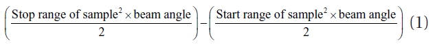
The data flow for a semiautomated analysis of DIDSON data is depicted in Fig. 1. First, a ddf file, which is a raw data file from the DIDSON system, was input into Echoview and converted from signal magnitudes to volume back-scattering strength (S_V) (step 1 in Fig.1 ). The data file contained background noise in the form of a stationary object, which may occur when the DIDSON system is set up in a fixed location. To remove the background noise, pings that did not contain fish echoes were defined by choosing a subset of pings that were considered pings with noise (step 2 in Fig.1 ). These subset pings were then averaged and subtracted from each data sample or pixel in each beam of every ping. This noise subtraction enhances the signal to noise ratio (step 3 in Fig.1 ). To improve target definition, namely multiple individual fish, a convolution (3Χ 3 median filter) was applied to the noise-removed echogram. This procedure smoothed the image of the targets without significantly affecting fish shape (step 4 in Fig.1 ). The next step of multibeam target detection was to identify clusters of above-threshold samples and reduce them to point data that include the geometric center, mean intensity, length, and other properties of each cluster. In other words, the cluster identified as a point was treated as a target or an individual fish (step 5 in Fig.1 ). In this study, the terms “target” and “fish” are used interchangeably. Each point has various target properties, which are characteristic of an individual fish. Several representative target properties are as follows. Length (cm) is the maximum distance between any two of the above threshold samples in the target. Thickness (cm) is the maximum range (interval) covered by the outline of samples per beam in the target. Area (cm²) is defined as the sum of the areas of all samples within the target boundary and can be expressed as:

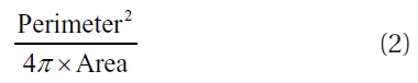
Perimeter (cm) is calculated as the sum of the target circumference contributions from the above-threshold samples in the target. Compactness is the inverse of the circularity ratio and is calculated (LeFeuvre et al., 2000) as:

[Fig.1.] The data flow of the semiautomated analysis of dual frequency identification sonar (DIDSON) data. The detailed explanations are found in the text. The number in black represents the order of each step taken to complete the data flow.

Orientation (^°) is the angle between the length derived axis and the line perpendicular to the transducer axis. The length axis was defined as the line joining the two most distant samples in the target. Orientation at 0^° means that a target is in a horizontal position, and 90^° indicates that the target is in a vertical position. The detected point targets were converted to a single-target data type for efficient visualization of target data across time (step 6 in Fig.1 ). That means that the conversion from a multibeam ping collapses into a single ping. Each column on the converted echogram represents a multibeam ping. This step permits the converted single-target echogram to act as an ordinary single-target detection echogram from a single or split beam echosounder. Each resulting single target has a range (the distance from a transducer to a target) and a major-axis (horizontal axis or athwartship axis) angle corresponding to the range and angle of a multibeam target. The single targets retain all of the above target properties. Entire single targets with target properties can be exported in the comma separated values (CSV) format and can be reimported (step 9 in Fig.1 ). Using the reimported CSV file, the calculation up to the converted single-target echogram was compacted to improve performance. The alpha-beta tracking algorithm (Blackman, 1986) was used on this single-target echogram to detect fish tracks. An aim of fish tracking is to obtain the numorgber of fish tracks, that is, the number of fish, and information related to fish behavior. The outcomes of fish tracks such as speed, changes in depth, and distributed depth can be exported in CSV format for further analysis. Here, the speed (m/s) was calculated as the accumulated distance between targets in a fish track divided by the total time. The change in depth (m) is the depth of the first target minus the depth of the last target in a fish track (Myriax, 2011).

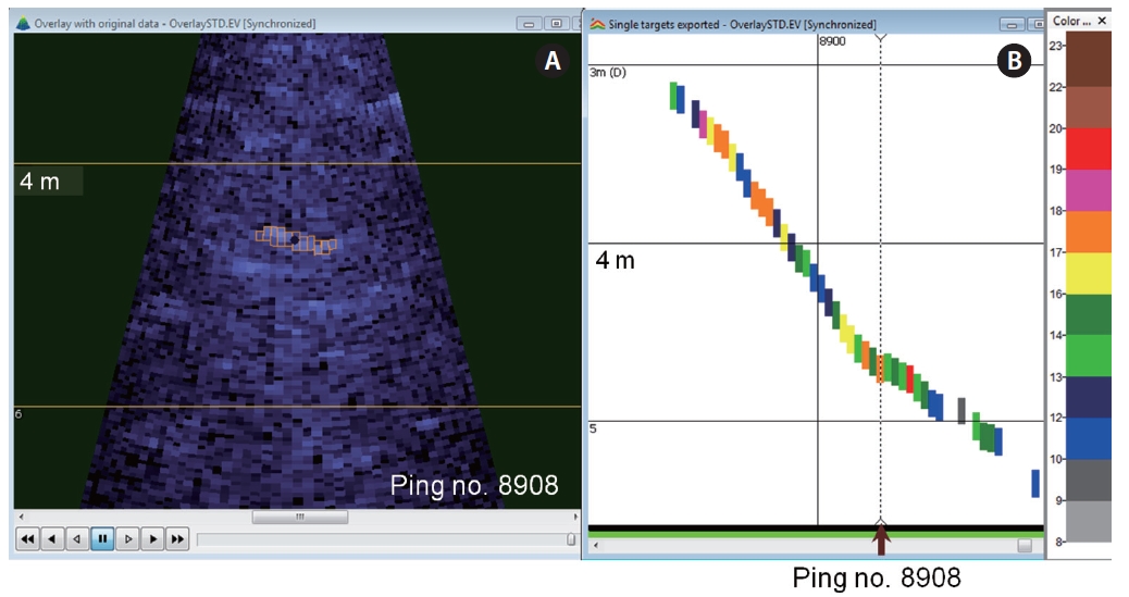
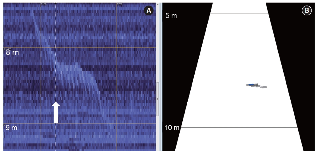
A multibeam echogram overlaid with targets helped to verify the targets detected (Fig.2 A). Data samples that contribute to the target are displayed with a highlighted outline. The fish-shaped echoes, highlighted in orange outlining multibeam target detection, are the detected targets (step 7 in Fig. 1 and Fig.2 A). The fish tracking technique was performed on the reimported single-target echogram (Fig.2 B) to elucidate fish behavior such as speed, depth, and changes in depth. A multibeam echogram synchronized with a single-target echogram, namely via looped multibeam replay, can be used to visually verify target validity. Any selected region on the single-target echogram can be viewed simultaneously with that region using the looped multibeam replay.

[Fig.2.] Echogram overlaid with detected targets (A). The fish shaped echoes with an orange outline are a target detected on a multibeam target detection (step 5 in Fig. 1). The re-imported single target echogram (B) created by exporting all single targets on the converted single target echogram as a comma separate values format and by re-inputting into Echoview. The multibeam echogram (A) and the single target echogram (B) are synchronized. The ping (A) which is the ping number 8908 is the same as the column with the dotted line (B). The single targets (B) can thus be verified by the comparison with targets on (A). The number on the solid vertical line (B) is the ping number and the solid vertical line is part of a grid set to every 100 pings on the echogram.

Single targets can be filtered from any target property using a threshold with a minimum or maximum value. For example, the single-target echogram (step 10 in Fig.1 ) was made by choosing targets located in the angle position between -10^° and 10^°, and the echogram was named “between -10^° and 10°.” Targets on the edge of the beam may not be completely ensonified. Therefore, selection by angle position can be exceedingly beneficial when only entire fish size is selected for analysis. The single-target echogram (step 11 in Fig.1 ) was created using a threshold (the maximum length of 35 cm) to define targets smaller than 36 cm, and the echogram was called “smaller than 36 cm.” The single targets were defined only if they were larger than 35 cm, which was the minimum threshold length (step 12 in Fig.1 ), and this echogram was called “larger than 35 cm.” The length of 35 cm was determined based on the proximity of the smallest length of the tar-

[Table 1.] Minimum maximum average and standard deviation of length and thickness substituted for targets in the “smaller than 36 cm” and “between -10° and 10°” echogram

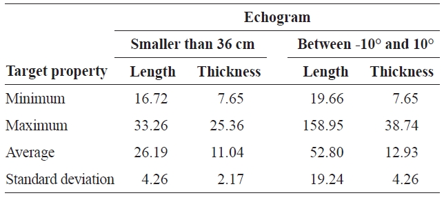
Minimum maximum average and standard deviation of length and thickness substituted for targets in the “smaller than 36 cm” and “between -10° and 10°” echogram

geted species. The mean intensity of a single target can be replaced with another target property for a better understanding and visualization of the target property. For example, length and thickness were substituted for intensity in the echograms “smaller than 36 cm” and “between -10^° and 10^°,” respectively. The minimum, maximum, average, and standard deviation of the length and thickness substituted in the targets of the echograms “smaller than 36 cm” and “between -10° and 10°” are shown individually in Table 1. The two echograms are examples of the usefulness of selecting by threshold and substitution.

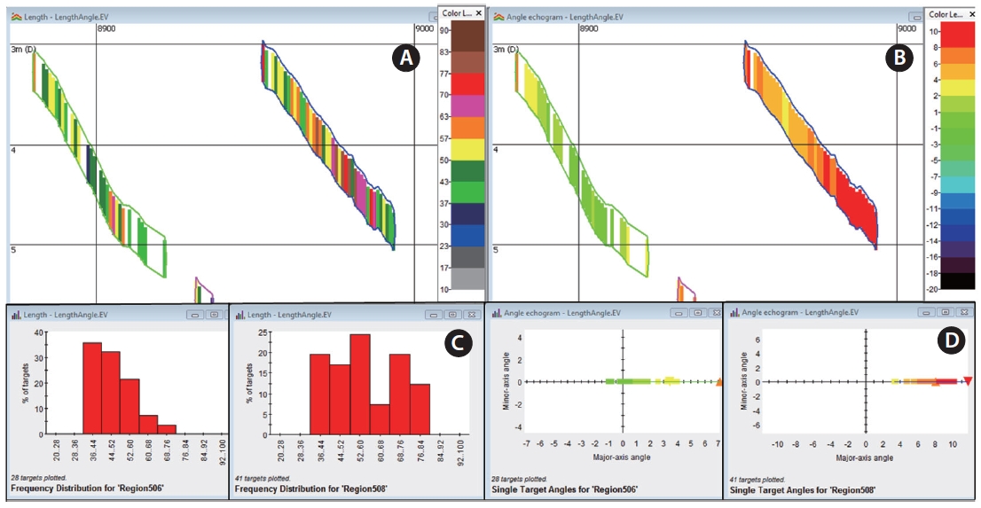
The substituted length and angle for the mean intensity on the “larger than 35 cm” echograms (step 13 and 14 in Fig.1 ) are illustrated in Fig. 3. The color-coded visualization assists in easily distinguishing the size and angle position of a target. The color denotes the representative length, and red and brown colors describe longer lengths than green and blue. Lengths of targets from the fish track on the left side are smaller than those on the right, according to the frequency distributions (Fig.3 C). Based on the graphs with major and minor-axes angles (Fig.3 D), which are downward views, the green targets indicate that they were placed on the left side of the beam angle, and red means that they were located on the right side of the beam angle. Note that the minor-axis angle is always zero, as the conversion to single targets from multibeam targets utilized only major-axis angles. The fish track on the right side (Fig.3 B and 3D) is located farther to the right

[Fig. 3.] Length echogram (A) and angle echogram (B) with two fish tracks. The color legend marks the length of the fish (A) and the angular position of the fish (B). The X axis is the depth displaying a horizontal line every 1 m. The Y axis is the number of pings representing every 100th ping. The frequency distributions of length from the two tracks (C) and the plots of angular positions which are looking downwards (D).

side of the beam angle compared to the fish track on the left. The direction of swimming fish, for example, downstream or upstream, can be understood using the angle information; if a target starts to appear at the edge (left or right) of the beam and to swim across the beam, then the target direction can be predicted with that information along with the fixed location of the transducer and the flow of the river. Additionally, fish tracks might be disrupted due to tidal stage and fish behavior, particularly when fish are swimming rapidly, so the tracks detected might need to be edited manually. The observation of the sequences of angles, that is, the color-display, on the angle echogram provides a clue as to whether a fish track is disrupted and whether it consists of one or two fish.

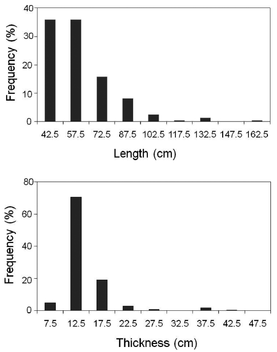
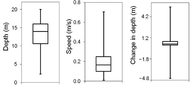
Various target properties of every single target were exported from the “larger than 35 cm” echogram. The total number of fish tracks was 248, which indicated the number of fish. The average values of representative target properties such as length, thickness, perimeter, compactness, and orientation were 59.8 cm, 14.0 cm, 193.9 cm, 3.6, and 109.4°, respectively. The frequency distributions of the lengths and thicknesses exported from the “larger than 35 cm” echogram are shown in Fig. .4 Lengths of 42.5 and 57.5 cm were dominant, and the thickness of 12.5 cm was clearly outstanding. The characteristics of fish behavior such as distributed depth, speed, and changes in depth are described using the boxplot in Fig. .5 Average and standard deviation values of depth, speed, and change in range were 13.12±4.21 m, 0.19±0.12 m/s, and 0.40±0.89 m, respectively. The half fish tracks were distributed at a depth between 10.6 and 16.1 m. The range of the third quartile of the speed and its maximum was relatively large at 0.46 m/s. Half fish tracks had a considerably narrow range of depth change, such as 0.03 and 0.52 m, although the minimum and maximum values were exceedingly small and individually large, i.e., -4.75 m and 5.43 m.

[Fig. 4.] Frequency distribution of length and thickness from the “larger than 35 cm” echogram which was created using a threshold with a minimum length of 36 cm.

[Fig. 5.] Boxplot of fish behavior characteristics of fish tracks from “larger than 35 cm” echogram. Fifty percent of the samples (box) and the first and third quartiles (bars) are shown.

Plotting the maximum intensity of all beams provides a fish tail-beat pattern, reflecting the size, shape, and swimming motion of the fish (Mueller et al., 2010). Mueller et al. (2010) found that the tail-beat frequency was 2.0-3.5 beats/s in sockeye salmon and 1.0-2.0 beats/s in chinook salmon. This technique was implemented in Echoview. An example of the maximum intensity echogram (step 8 in Fig.1 ) is illustrated in Fig. .6 The maximum intensity echogram depicts the fish swimming pattern in the shape of caterpillars with legs extending to one side. The caterpillar pattern results from periodic changes in the range extent of the fish echoes. A sequence of caterpillar legs concurs with the location of the tail within the tail-beat cycle. Therefore, the time interval between consecutive legs is related to the tail-beat frequency, which may be beneficial for studying acoustic species identification and bioenergetics.

[Fig. 6.] Echogram of tail-beat pattern. The ping number of 1119 was marked by a white arrow on the single target echogram (A step 8 in Fig.1 ) and is the current ping on its corresponded image smoothed echogram (B step 4 in Fig.1 ).

The data flow of the semiautomated analysis (Fig. 1) can be used as a template. When new data files are input into Echoview, the data flow template can be applied to these new data sets. Thus, manually creating data flow may not be necessary. However, the parameter settings for the semiautomated analysis must be modified according to the characteristics of the data and the aim of the research. The data flow of the semiautomated analysis can be varied according to the needs of the research. This methodology can also be applied to data from the BlueView two-dimensional imaging sonar (Blue-View Technologies, Seattle, WA, USA). This sonar operates at lower frequencies (450 and 900 kHz) than that of DIDSON and provides a wide field of view (45-50^°) and a longer maximum range of 137 m, but resolution is lower than that of DIDSON due to wider beam widths. Imaging sonars have some limitations. The image is dependent upon the density and surface area presented by an object to the sonar. Therefore, when a fish turns directly toward or away from the imaging sonar, it will sometimes be lost from view. Certain fish species can be identified based on their outlines and swimming patterns. Hence, distinguishing species becomes difficult unless clear and consistent differences exist in size or behavior. The length of echoes of a fish crossing through a ping is related to its depth because of the beam spreading effect. Thus, the length of crossed fish echoes at shallower depths is shorter than that at deeper water depths. Therefore, the above-mentioned points should be considered when collecting data.

Fish tracking using DIDSON data in Echoview is like using well-defined fish movements, as having major-axis angles, each with a very accurate position, provides better results than major and minor-axes angles in which relative positional inaccuracy occurs. Therefore, it often requires little editing of tracks because the across-fan angle is well-defined and very consistent compared to split-beam data.

An automated tracking method, which is similar to the method of tracking by Echoview, has been introduced (Handegard and Williams, 2008). The tracking algorithm was coded in Matlab (MathWorks, Novi, MI, USA), which has been very widely used among scientists. However, handling a vast volume of data with a high processing speed is not easy. The algorithm can be divided into target detection and target tracking. In target detection, the processes of noise removal, thresholding, and image convolution filtering were the same as those of Echoview. However, different approaches were used to calculate target position. The target position was at the geometric center of the target in Echoview, whereas an intensity-weighted position was used in the study by Handegard and Williams (2008). In particular, they implemented range-dependent filtering, which compensated for beam spreading and fragmentation within a short range. The multiple-target tracking algorithm and the auction algorithm have been used for target tracking (Bertsekas, 1990; Blackman and Popoli, 1999) and are also employed in Echoview (Blackman, 1986; Bertsekas, 1990). Their tracking algorithm was designed primarily for studying fish behavior rather than for fish counting and sizing. Accordingly, their tracker offered fish speed and direction as an outcome. However, range-dependent filtering was an advanced feature, which may be implemented in Echoview in the future. Another study on an automated method for counting fish and estimating their size using DIDSON data was published (Han et al., 2009). This method was performed as a trial stage for yellowtail Seriola quinqueradiata, while fish were being transferred between cages within a fish farm. Two new techniques, a phase-only correlation for stabilizing images from a moving net and a running Gaussian average for subtracting the background noise, were used. A different tracking algorithm from that used by Echoview was utilized. The Kalman filter algorithm was adapted to track fish movement in their study, whereas an alpha-beta fixed gain filter was used in Echoview. The alpha-beta tracker would work better under multiple target conditions than the Kalman filter. However, a direct comparison between the two algorithms using the same data set would be required to assess performance more precisely. Han et al.’s (2009) trial method was built for fish counting and sizing, so it provided the number and length of the fish, but did not provide information on fish behavior. Hereby, Echoview is of great advantage for those interested in fish counting, sizing, and studying fish behavior.