검색 전체 메뉴
PDF
맨 위로
OA 학술지
Analysis of Scaling Parameters of the Batch Unscented Transformation for Precision Orbit Determination using Satellite Laser Ranging Data
  • 비영리 CC BY-NC
  • 비영리 CC BY-NC
ABSTRACT
Analysis of Scaling Parameters of the Batch Unscented Transformation for Precision Orbit Determination using Satellite Laser Ranging Data
KEYWORD
precision orbit determination , batch unscented transformation , scaling parameter , satellite laser ranging system , TOPEX/Poseidon
  • 1. INTRODUCTION

    Determining the orbit of satellites more accurately has become a much more significant objective. In terms of precise satellite tracking technology, satellite laser ranging (SLR) holds the normal point (NP) accuracy of mm,and the accuracy of single shot in cm (Montenbruck &Gill 2000). With this high level of accuracy, SLR can be easily applied to the independent revision of other satellite tracking systems, and is used in various fields of application, such as verifying the effectiveness of the Global Navigation Satellite System (GNSS), space geodesy, the Earth’s gravitational field, displacement of the Earth's crust and geodynamics (Zhu et al. 1997, Biancale et al.2000, Urschl et al. 2007). For the high accuracy of the SLR system in order to more precisely fulfill the function of determining the orbit of a satellite, an accurate kinematic model and the existence of an observation model that minimizes error become important elements. Satellite orbit determination software is largely composed of the dynamic model, observation model and filtering algorithm. To precisely determine the orbit of a satellite, it is necessary not only to model the elements that influence the motions of the satellite, but also to model the environmental factors according to observation data and equipment when gaining the tracking data of the satellite,and reflecting those results in the process of calculation.It is also very important to choose a filtering algorithm for the process of minimizing the residual between actual observation values and calculated observation values.

    In filtering algorithms used for orbit determination, there is the consecutive method that is enabled for real-time estimation, and a batch processing method based on the principles of the least-squares method that uses the data observed in the past. Both of these filtering algorithms have the following restrictions when using the SLR data. First, since there are currently about 40 SLR satellites and about 50 SLR ground stations around the world, the amount of SLR data is not sufficient. Second, since it is difficult to continuously track satellites due to the small number of satellites and ground stations, such an approach has the disadvantage of being unsuitable for real-time processing. Finally, the dispersion of discontinuous data means that there are ways in which errors may be induced, or the functions of filters restricted. For this reason, based on processing the data through the batch processing method, the batch unscented transformation method (Park et al. 2007) is applied to overcome the error elements that result from the small amounts of data and the discontinuous data dispersion. The unscented transformation that becomes the foundation of the batch unscented transformation method is the method of predicting the mean and covariance from the non-linear system. Since it uses the sigma points of specific numbers and does not use the random sampling of the Monte Carlo method, it is possible to gain the maximum results in a short period of time (Julier 2002, Julier & Uhlmann 2002).

    The state of the sigma point is initially created, which influences the accuracy of orbit estimation when using the batch unscented transformation method for the precision orbit determination (POD). To determine the state of the sigma point, the initial covariance and the scaling parameter are required (Howlett et al. 2004). Deciding how to set the scaling parameters influencing the resolution of the sigma points will change the results of the estimation algorithm, and furthermore will contribute to increasing the accuracy of orbit determination. In other words, according to the scaling parameters in the batch unscented transformation method, the precision and the convergence performance of the orbit determination may be changed. The scaling parameters α, β, κ, λ influence the formation of the sigma point in the process of unscented transformation, and play a significant role in the orbit determination algorithm. Each of the scaling parameters has a different level of influence on the generation of sigma points. Each scaling parameter influences the formation of all sigma points with certain degree of differences through the unscented transformation process. The scaling parameter can play the main role in the orbit determination and sigma point generation. Then, the scaling parameter must be taken carefully to its application.Thus far, the research on the correct roles of the scaling parameters and their contributions to orbit determination using the batch unscented transformation method has been insufficient. The main purpose of the current research is to realize the roles of scaling parameters and their contributions to the unscented transformation in precision orbit determination using SLR data.

    2. BATCH UNSCENTED TRANSFORMATION

    In this section, batch unscented transformation (Park et al. 2010) is briefly reviewed to explain the scaling parameters in the process. The batch processing method estimates the states by using overall observation data in a selected orbit section. Meanwhile, the sequential processing method estimates the states within each of the observation times. Within the sequential processing method with no process noise, the algorithms between the methods hold a mathematical similarity. Therefore, the typical unscented Kalman filter (UKF) is very useful in materializing the new batch unscented transformation method (Park et al. 2010). The batch unscented transformation method for orbit determination has the following assumptions. If observational noise can be considered a fixed value, the algorithm can be derived from the Kalman filter. Therefore, the state and covariance are expressed in the following Eq. (1) for the UKF,

    image

    where xTk represents the unobserved state of the system, vTk is a process noise, nTk is observation noise, and the prediction of the covariance of xk is given by Pak (Wan & van der Merwe 2001).

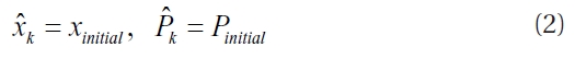
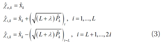
    First, when assuming the estimation for the covariance with the initial state with Eq. (2) to obtain the sigma point, it is as displayed in Eq. (3), where L is a dimension of augmented state and λ is a composite scaling parameter.

    image
    image

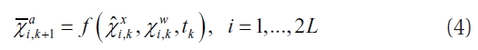
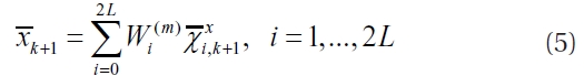
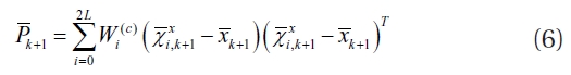
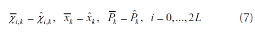
    In the UKF, the states are propagated to the following observation time to renew into a greater value through the non-linear dynamic model Eq. (4). However, since the batch unscented transformation filter uses all of the values observed during the entire period to accomplish the estimation, the sigma points propagated are the same as the estimated values of the past. Therefore, Eqs. (4-6) do not have to be calculated, and the propagated state and the covariance within the chosen time can change as in Eq. (7).

    image
    image
    image
    image

    The sigma points (χt,k(t=0,...2L)),= selected at the specific times are propagated out to calculate for the overall observation value. Each of the sigma points are propagated out, and the observed vectors are calculated according to each of the observation times (tj,)=1,...,,N,j≠k) through the non-linear observation model and are expressed as shown in the following equation.

    image

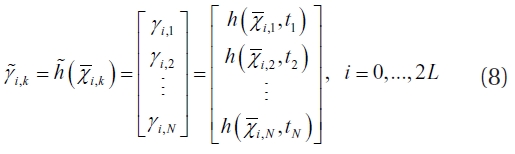
    The χi,j(i,e. χi,1χi,2,..,χi,N) on the right term of Eq. (8) are the sigma points propagated (tj,j=1,...,N,j≠k) from each of the observation times, while N is the overall number of the observation times. The propagated covariance and observations within the observation times are calculated as shown below.

    image
    image
    image

    Rk is the matrix of observation noise, the mutual correlation matrix is as shown in the following Eq. (11), and the profit matrix is defined as shown in Eq. (12).

    image

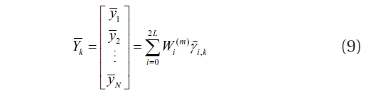
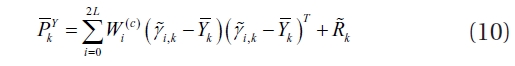
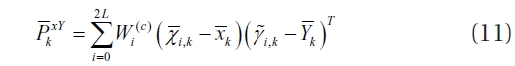
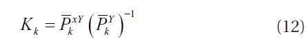
    Finally, the state in time
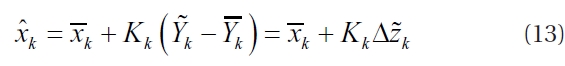
 tk is renewed according to Eq. (13).

    image
    image

    Here, ΔZK is the observation residual matrix that is the difference between the calculated value Yk and the actual observed value Yk for the overall observation time. The batch unscented transformation filter algorithm from Eq. (9) to Eq. (13) is similar in form to the unscented Kalman filter algorithm, but has several differences. If the number of the different forms of observations is nmeas then the total number (Ntot) of the observation data is nmeas × N . The degree of the observation matrix (yk) and the covariance matrix (PYk) of Eq. (9) and Eq. (10) each become Ntot × 1 and Ntot× Ntot. From Eq. (11) to Eq. (13), the dimensions of the mutual correlation matrix (PkxY) and the profit matrix (KK) are both L × Ntot. From Eq. (2), the initial states use Eq. (13) for correction and renewal. The loop will stop iterating when the requirement of the least squares method is equal to Eq. (14) (Vallado & McClain 2001).

    3. SCALING PARAMETERS IN THE BATCH UNSCENTED TRANSFORMATION

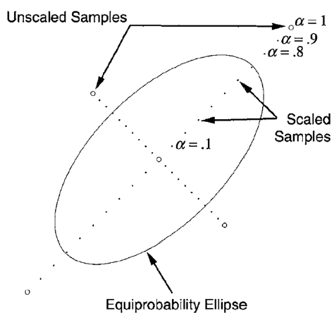
    First of all, setting the scaling parameters in the batch unscented transformation affects the precision and the convergence performance of the orbit determination, because the scaling parameters influence the formation of the sigma point in the process of unscented transformation. Accordingly, it can be observed that the scaling parameters play an important role in the process of orbit determination. The unscented transformation becomes a basic process for the batch unscented transformation method, and the transformation evaluates the mean and covariance from the non-linear system. The batch unscented transformation is similar to the Monte Carlo method with numerous sigma points, but it does not use numerous sigma points randomly but rather uses the sigma points described in Eq. (2) for a smaller sigma point. In general, the sigma points are composed of one mean and covariance, which are determined by the number of dimensions. The scaling parameter concept of unscented transformation is a further application of the symmetric unscented transformation that allows some sampling and weighting adjustments to improve strength against higher order non-linearities. It uses four adjustable scaling parameters α, β, κ, λ to allow for some setting of the unscented transformation for specific uses.

    Suppose x has mean x and covariance Px. According to the Eq. (3) forming a matrix χ of 2L + 1 sigma vectors, λ = α2 ( L+ κ ) ? L is a scaling parameter (L is the number of dimensions). In general, the scaling parameter α which determines the spread of the sigma points around x is usually set to a small positive value ( e.g., ≤ α ≤ 1), scaling parameter β is used to incorporate prior knowledge of the distribution of x ( e.g., β0) and secondary scaling parameter kappa is usually set to 0 or 3-L (Julier et al. 1995). For example, new sigma points x'i ( i = 0,..., 2L ) in Eq. (3) can be obtained by adding χ0 and α (χiχ0), which multiplies the subtractions of the sigma points (χ0 and χi (i = 0,..., 2L)) by the scaling parameter α, as follows:

    image

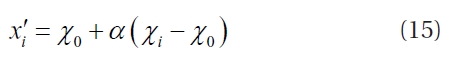
    The sigma points can be scaled towards and away from the mean of the prior distribution by appropriately selecting κ. As dimension L increases, the radius of the sphere that bounds the sigma points increases as well. Simultaneously, higher order effects become more significant as the dimension increases. So, Eq. (15) overcomes dimensional scaling effects by calculating the transformation of a scaled set of sigma points of the form, where α is a positive scaling parameter that can arbitrarily be made small to minimize higher order effects.

    The positive scaling parameter α and the secondary scaling parameter κ can be combined into scaling parameter
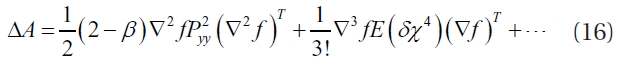
 λ, which determines scales among the sigma points. So, scaling parameter λ is weaker than the other scaling parameters in terms of its influence. Also, the value of scaling parameter κ can be found through the equation L+ κ = 3, because for any choice of κ, the first, second, and third order moments of the sigma point distribution are fixed, but the fourth order moment is scaled by L+ κ, which is given by 3 (Julier & Uhlmann 2002). Therefore, the unscented transformation actually uses three adjustable scaling parameters α, β, κ. The scaling parameter α is a positive value used for an arbitrary small number to a minimum of higher order effects. The scaling parameter α obeys the two laws as follows. First, it must be defined as a positive semidefinite. In addition, second order accuracy must be maintained about the mean and covariance after calculation (Wan & van der Merwe 2001). The effect of the scaling parameter α on the samples is illustrated in Fig. 1 for a Gaussian distribution. Due to the effect of the scaling parameter α, scaled samples that were referenced as sigma points can be distributed, such as in Fig. 1. In general, the scaling parameter κ, which is a secondary scaling parameter, is determined by the number of dimensions. Therefore, the positive scaling parameter α and the third scaling parameter β become the scaling parameters that play the most important role. The unscented transformation can be extended to include partial higher order information of the fourth order term in the Taylor series expansion of the covariance. The third scaling parameter β can be found a value of constant as shown in Eq. (16) below (Julier 2002).

    image

    Here, ΔA is predicted covariance error in the fourth order term, β is the third scaling parameter, f is non-linear transformation through the Taylor series expansion, x is N-dimensional random variable, y is the result of the non-linear transformation of x, Pyy is the covariance of y, and E is expectation value. According to Eq. (16), ΔA term has minimum value when β has constant value (Julier 2002). In short, if the number of dimensions is known, κ is directly determined, and λ can be found when α is chosen. By confirming through Eq. (16), the scaling parameter β is also found to not be a factor that has a great impact, and therefore, the current study will focus on the scaling parameter α to gain the optimized POD.

    4. SIMULATIONS AND DISCUSSIONS

    The purpose of the present study is to investigate the roles of scaling parameters of the batch unscented transformation method for the POD of a satellite using the SLR observation data. The dynamic equation is composed using Cowell's method (Vallado & McClain 1997), and the observation data is actual TOPEX/Poseidon SLR data. The Earth gravitational model 1996 (EGM96) (Lemoine et al. 1998) is used for the numerical model for the Earth's asymmetrical gravitational field, and the Jacchia 71 model (Lyndon 1982) is used as the density function to calculate the atmospheric refraction (Marini & Murray 1973). Moreover, the perturbations by the gravitation of the Sun and the Moon and the perturbation of the Sun's radiation pressure are considered, and the Earth’s crust and tidal force from the Sun and the Moon are also considered. For the numerical integration of the dynamic model, the Adams-Cowell method, one of the multi-step methods, is used. The observation model postulates the 4 ground observatories positioned on the surface of the Earth (McDonald, Monument, Borowiec, Herstmonceux), and utilizes the range data between the satellite and the ground observatory observed from each of the observatories as the observation data. As the filtering algorithm, the batch unscented transformation filter is applied. When using the batch unscented transformation method, the scaling parameters affect the precision and the convergence performance of the orbit determination. It can be observed that the scaling parameters play an important role in the process of orbit determination. Four adjustable scaling parameters α, β, κ, λ are considered to form an appropriate setting of the unscented transformation mentioned in Section 2. In the estimation process, the scaling parameters were assigned sequentially for the orbit determination algorithm. The scaling parameters that showed the best results were selected in terms of range residual.

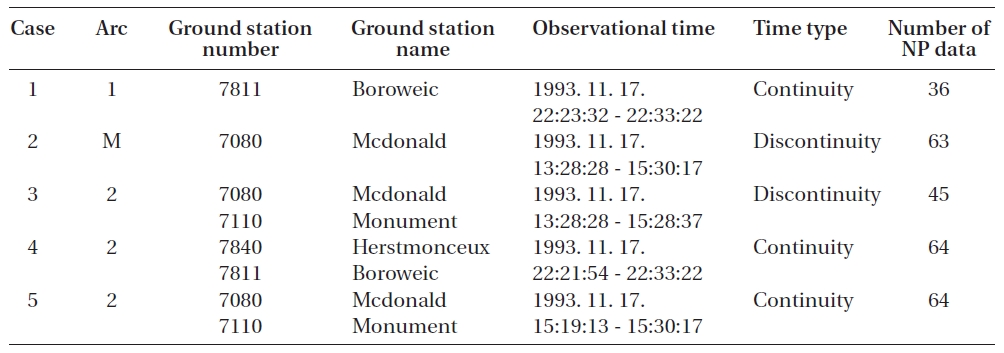
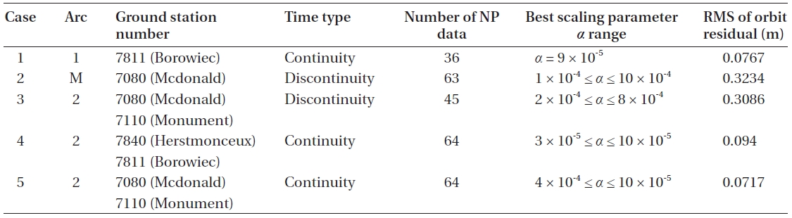
    [Table 1.] The ground station and observational data information.

    label

    The ground station and observational data information.

    To verify the precision orbit determination, the results of the orbit determination are compared with ephemeris by Jet Propulsion Laboratory1 (JPL) that are assumed to be true orbits. The official ephemeris of TOPEX/Poseidon was calculated through the differential global positioning system (DGPS) method using the global positioning system data (Melbourne et al. 2007). The POD error with DGPS method is approximately 2 cm RMS on the radial direction (Bertiger et al. 1994, Schutz et al. 1994, Yunck et al. 1994).

    The paper attempts to simulate four types of tests depending on the characteristics of the observatories from arc information of Table 1, which include arc number, ground station number, ground station name, observational time, time type, and the number of normal point data. The orbit determination results are composed of no initial position error, 10 m error, 100 m error, and 1 km error of initial position, respectively. Here, the position errors are computed for radial, along, and cross direction. To verify the self performance of the POD, the orbit determination is performed when the initial state error was 0. The initial state is composed of position and velocity from the interpolation value of ephemeris on epoch time by JPL. The simulation results consist of four kinds of cases that depend on the observational data type. To find the appropriate scaling parameters, the simulations are performed for four cases, such as case 1 (applying one arc to one base station), case 2 (applying multi-arc to one base station), case 3 (applying two arcs from discontinuous observation time for two base stations) and case 4 (applying two arcs from continuous observation time for two base stations).

    In this research, the number of dimensions L = 6 is known because position vector and velocity vector of the satellite are set as estimation states. As mentioned earlier, the range of scaling parameter α is 0 ≤ α ≤ 1, scaling parameter β is set as β = 2, scaling parameter κ is set as L+ κ = 3, and scaling parameter λ is obtained from λ = α2 ( L+ κ ) ? L. κ is directly determined as κ = ?3. When α is chosen, λ can be found through λ = 3α2 ?6. The length of each interval of the scaling parameter α is divided by 10-4 or 10-5 unit to find the appropriate value in the orbit determination algorithm, because the scaling parameter α must be defined as a positive semidefinite and close to zero. If the scaling parameter α is greater than 10-4 or less than 10-5, most of the results of the orbit estimation will diverge, because the scaling parameters chosen for the present estimation are not suitable. The most common criterion for showing the error between true orbit and estimated orbit is the range residual. The error is the calculated RMS value from difference between the calculated range and measured range, which is expressed by Eq. (17). In the equation, Xmeas is a measured range value, Xest is a calculated range value, and N is the number of observation data. However, this criterion is not perfectly reliable in terms of reflecting the accuracy of orbit determination.Although the residual of range is a very small value, actual orbit estimation accuracy can be larger than the range residual. For this reason, the accuracy of the orbit determination is shown by position vector error in radial, along, and cross direction by comparing true orbit and estimated orbit in this research.

    image

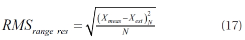
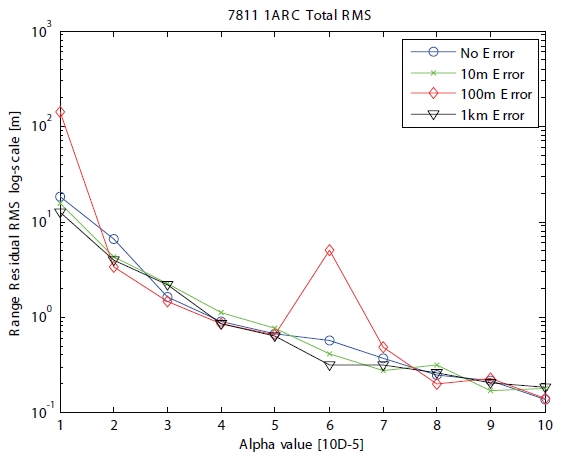
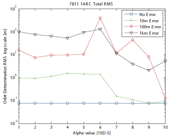
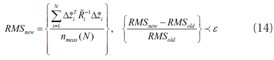
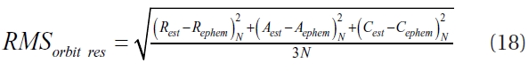
    Case 1 applies one arc to one ground station (Boroweic).The initial orbit elements are given as position and velocity vectors. The number of total iterations is ten for the batch unscented process. The iteration process is stopped when the iteration number reaches a total iteration number, or when the gap of previous and present RMS errors is smaller than the arbitrary convergence criterion(2 × 10⁻²) chosen to maintain the best performance of the simulation. The values of initial position covariance and velocity covariance are fixed as 10-2 m and 10-8 m/s respectively, because they are similar to the errors of initial orbit elements from ephemeris. Moreover, the initial velocity covariance is generally less than the initial position covariance (Park et al. 2007). The information of observational data and ground station for case 1 is shown in Table 1. Strictly speaking, the time type of case 1 is similar to continuity. True position refers to the actual satellite position from the precision orbit ephemeris (POE) by JPL, and the estimated position is obtained from the final value of POD. The orbit residual is calculated from the difference between the true position and the estimated position as the RMS represented by following equation. Here, Rest is an estimated position of radial direction, Rephem is a true position of radial direction from ephemeris, Aest is an estimated position of along direction, Aephem is a true position of along direction from ephemeris, Cest is an estimated position of cross direction, Cephem is a true position of cross direction from ephemeris, and N is the number of observation data obtained from all observation points.

    image

    The RMS of range residual shown in Fig. 2 according to the positive scaling parameter α varies from 1 × 10⁻⁵ to 10 × 10-5. No Error means that the initial conditions of the position take the same value of the true orbit (POE) at the epoch time in the figure. The initial position imposes 10 m error, 100 m error and 1 km error from the true orbit (POE) at the epoch time, respectively, when initial velocity has no errors. The RMS of range residual is about 10 cm when scaling parameter α varies from 7 × 10⁻⁵ to 10 × 10-5 in Fig. 2. For a critical comparison, the orbit residuals are required. Fig. 3 shows the 3-dimensional (3D) RMS of orbit residuals which are compared to the POE by JPL. The RMS of orbit residual is about 8 cm error with no initial position error at the epoch time, 50 cm error with 10 m initial error, 10 m error with 100 m initial error, and 10 m error with 1 km initial error. Satisfactory orbit determination results could not be obtained when the initial error was 100 m or 1 km, because the number of observation data was not sufficient. Accordingly, the research

    focused on tuning the scaling parameter when the initial error was 10 m. When the scaling parameter α is 9 × 10-

    5, the RMS of orbit residual in the case of 10 m position error is about 8 cm, which is a similar result to no initial position error.

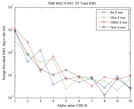
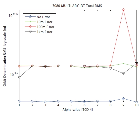
    Case 2 is applied for multi-arc to one ground station, and is shown in Table 1. The time type of case 2 has discrete characteristics. The initial position errors are assumed as none, 10 m, 100 m and 1 km. The RMS of range residual shows in Fig. 4 according to the positive scaling parameter α varies from 1 × 10⁻⁴ to 10 × 10-4. The RMS of range residual yields about 8 cm when α has from 4 × 10⁻⁴ to 10 × 10-4 in Fig. 4. Fig. 5 includes the 3-dimensional RMS of orbit residual errors, which are compared to the POE by JPL. The orbit residuals show about 30 cm error with no initial position error, 10 m initial error, 100 m initial error, and 1 km initial position error, except when the scaling parameter α is 9 × 10⁻⁴. According to the results, α = 9 × 10⁻⁴ is not the fine tuning value for this orbit determination algorithm.

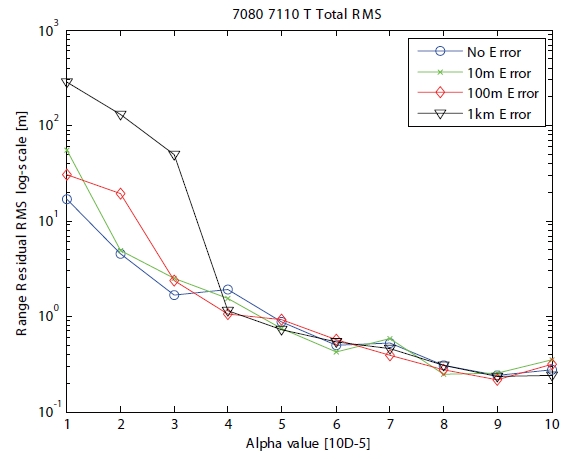
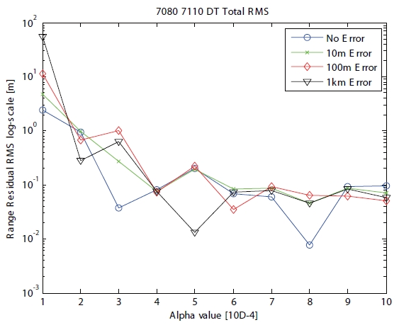
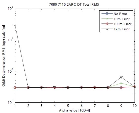
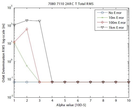
    Case 3 is applied for two arcs to two ground stations, and is presented in Table 1. The time type of case 3 has discrete characteristics with different observation times in two ground stations. The RMS of range residual is shown in Fig. 6 when the positive scaling parameter α varies from 1 × 10⁻⁴ to 10 × 10-4. The RMS of range residual is about 10 cm when α is from 4 × 10⁻⁴ to 10 × 10-4 in Fig. 6. Fig. 7 shows the 3-dimensional RMS orbit residual errors compared with the POE by JPL. The orbit residuals are about 20 cm for all of the initial position errors, when the scaling parameter α is from 2 × 10⁻⁴ to 8 × 10⁻⁴.

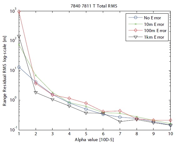
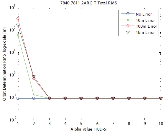
    The information of observational data and ground station in Table 1 is provided for case 4 applied to two arcs to two ground stations. The observation time of case 4 has a continuous attribute with the same time in two ground stations. In other words, the observation method of case

    4 means that two ground stations observe the same target at the same time. The RMS of range residual shown in

    Fig. 8 as the positive scaling parameter α varies from 1 × 10⁻⁵ to 10 × 10-5. The RMS of range residual is about 20 cm when α is from 6 × 10⁻⁵ to 10 × 10-5 in Fig. 8. Fig. 9 shows the 3-dimensional RMS of orbit residual errors compared with the POE by JPL. The orbit residuals have about 9 cm error for all initial position errors when the scaling parameter α varies from 3 × 10⁻⁵ to 10 × 10-5.

    Case 5 is applied for two arcs with two ground stations, and is presented in Table 1. The time type of case 5 has continuous features, with the same observation time in two ground stations. The RMS of range residual is shown in Fig. 10 when the positive scaling parameter α varies from 1 × 10⁻⁵ to 10 × 10-5. The RMS of range residual is about 20 cm when α is from 8 × 10⁻⁵ to 10 × 10-5 in Fig. 10. Fig. 11 shows the 3D RMS orbit residual errors compared with the POE by JPL. The orbit residuals are about 7 cm error for all of the initial position errors, when the scaling parameter α is from 4 × 10⁻⁵ to 10 × 10-5.

    Table 2 provides the summarized information of simulation results, including arc number, ground station number and RMS of orbit residual according to the range of the best scaling parameter α. It is found that changes in the scaling parameter have less impact on two-arc or multi-arc cases (cases 2-5) than on single arc (case 1), because two arc cases have a wider range of the scaling parameter α than the single arc case. More precise results can be obtained when the observation data are processed in continuous periods. If the observation data does not occur in the middle of observation, the accuracy of orbit determination will be reduced by uncertainties from the error occurring at this time. According to case 1, case 4 and case 5, the value of scaling parameter α tends to be selected as a small value when the observation data exists as a continuous time type (α = 9 × 10⁻⁵). The reason for the small value of the scaling parameter α selection is as follows. If the observation data are obtained continuously, the uncertainties due to the error will be comparatively smaller than the case of discrete observation data. Therefore, the sigma point distribution range will be small, and small scaling parameters are a better choice for the accuracy of orbit determination. On the other hand, if the observation data exists as a discontinuous time type, a larger scaling parameter α is required (2 × 10⁻⁴α ≤ 8 × 10⁻⁴) than the value of the scaling parameter in continuous cases. In other words, the value of the best scaling parameter α, which was found to be 10-4 with discontinuous two arcs and multi-arc, was larger than the value of the best scaling parameter α, which was found to be 10-5 with one arc and continuous two arcs. In addition, other characteristics can be found. Although one arc is sensitive to determine the scaling parameter, it is possible to elicit states holding high accuracy in accordance with the proper tuning conditions. Consequently, the RMS orbit residual error is found to have a level of accuracy within several cm (7.17 cm) in two arcs of McDonald and Monument ground stations. Accuracy of orbit determination

    [Table 2.] The best range of scaling parameter α.

    label

    The best range of scaling parameter α.

    algorithm in one arc of Borowiec station with an appropriately tuned scaling parameter α = 9 × 10⁻⁵ is also found to be within a few cm of the RMS orbit residual error (7.67 cm).

    In conclusion, more precise results were gained when the observation data existed as a continuous time type, and the value of scaling parameter α tends to be selected as a small value (α = 9 × 10⁻⁵) in the case of continuous time type. Although the use of just one arc does not provide enough observation data, the discontinuity of the observational data is low, and the optimal convergence value also exists in the small value of scaling parameter α, because sigma point distribution range is small. In contrast, when the observation data is a discontinuous time type, a larger scaling parameter α is required (2 × 10⁻⁴α ≤ 8 × 10⁻⁴).

    1ftp://podaac-ftp.jpl.nasa.gov/allData/topex/ [cited 6 May. 2010]

    5. CONCLUSIONS

    The values of scaling parameters in the batch unscented transformation method can change the accuracy and the convergence performance of the orbit determination.The purpose of this research was to determine the roles and contributions of the scaling parameters in orbit determination using the batch unscented transformation method. The major factor of orbit determination within the batch unscented transformation method is the state of the initial sigma points made from the scaling parameters. The physical meaning of the scaling parameters is a numerical value that determines the distribution and range boundary of sigma points. Thus, the scaling parameters are analyzed in order to understand their physical meaning for POD using SLR data. The appropriate scaling parameters are determined, and the tuning properties of the scaling parameters are analyzed for several observation data. Rather than the empirical value of the scaling parameters, the generally acceptable range of the scaling parameters is considered to improve the accuracy of the orbit determination algorithm. The process of creating the sigma points affects the accuracy and converging performance. Errors can be minimized by appropriately tuning the scaling parameters. Therefore, the fine tuning of the scaling parameters can improve the accuracy of the orbit determination results from the TOPEX/Poseidon SLR observation. If you use the batch unscented transformation method with other types of tracking data, the task of finding the appropriate scaling parameter must be carried out first. In this research, it is confirmed that the distributed range of the sigma points is strongly formed by the scaling parameter alpha, which is one of the applied factors within the converging performance of the orbit determination system.

참고문헌
  • 1. Bertiger WI, Bar-Server YE, Christensen EJ, Davis ES, Guinn JR 1994 GPS tracking of TOPEX/POSEIDON: results and implications [JGR] Vol.99 P.24449-24464 google cross ref
  • 2. Biancale R, Balmino G, Lemoine J-M, Marty J-C, Moynot B 2000 A new global earth’s gravity field model from satellite orbit perturbations: GRIM5-S1 [GeoRL] Vol.27 P.3611-3614 google cross ref
  • 3. Grewal MS, Andrews AP 2008 Kalman filtering: theory and practice using MATLAB P.330-344 google
  • 4. Howlett P, Pudney P, Vu X 2004 Estimation train parameters with an unscented Kalman filter in Proceedings of the Fifth Asia Pacific Industrial Engineering and Management Systems Conference Gold Coast Australia P.34.13.1-34.13.10 google
  • 5. Julier SJ 2002 The scaled unscented transformation in Proceedings of the American Control Conference Anchorage AK P.4555-4559 google
  • 6. Julier SJ, Uhlmann JK, Durrant-Whyte HF 1995 A new approach for filtering nonlinear systems in Proceedings of the American Control Conference Seattle WA P.1628-1632 google
  • 7. Julier SJ, Uhlmann JK 2002 Reduced sigma point filters for the propagation of means and covariances through nonlinear transformations in Proceedings of the American Control Conference Anchorage AK P.887-892 google
  • 8. Lemoine FG, Kenyon SC, Factor JK, Trimmer RG, Pavlis NK 1998 The development of the joint NASA GSFC and NIMA geopotential model EGM96 NASA Goddard Space Flight Center technical manual google
  • 9. Lyndon B 1982 Jacchia-Lineberry upper atmosphere density model NASA Johnson Space Center contract report google
  • 10. Marini JW, Murray CW 1973 Correction of laser range tracking data for atmospheric refraction at elevations above 10 degrees NASA Goddard Space Flight Center technical report google
  • 11. Melbourne WG, Davis ES, Yunck TP, Tapley BD 1994 The GPS flight experiment on TOPEX/POSEIDON [GeoRL] Vol.21 P.2171-2174 google cross ref
  • 12. Montenbruck O, Gill E 2000 Satellite orbits: models methods and applications P.202-228 google
  • 13. Park E-S, Park S-Y, Roh K-M, Choi K-H 2010 Satellite orbit determination using a batch filter based on the unscented transformation [Aerosp Sci Technol] Vol.14 P.387-396 google cross ref
  • 14. Park E-S, Roh K-M, Park S-Y, Choi K-H 2007 Satellite precise orbit determination using a new batch least squares in AAS/AIAA Astrodynamics Specialist Conference Sedona AZ google
  • 15. Schutz BE, Tapley BD, Abusali PAM, Rim HJ 1994 Dynamic orbit determination using GPS measurements from TOPEX/POSEIDON [GeoRL] Vol.21 P.2179-2182 google cross ref
  • 16. Urschl C, Beutler G, Gurtner W, Hugentobler U, Schaer S 2007 Contribution of SLR tracking data to GNSS orbit determination [AdSpR] Vol.39 P.1515-1523 google cross ref
  • 17. Vallado DA, McClain WD 2001 Fundamentals of astrodynamics and applications P.489-564 google
  • 18. Wan EA, van der Merwe R, Haykin SS 2001 The unscented Kalman filter in Kalman filtering and neural networks P.221-269 google
  • 19. Yunck TP, Bertiger WI, Wu SC, Bar-Sever YE, Christensen EJ 1994 First assessment of GPS-based reduced dynamic orbit determination on TOPEX/Poseidon [GeoRL] Vol.21 P.541-544 google cross ref
  • 20. Zhu SY, Reigber C, Kang Z 1997 Apropos laser tracking to GPS satellites [JGeod] Vol.71 P.423-431 google cross ref
이미지 / 테이블
  • [ Fig. 1. ]  Scaled sample points of scaling parameter α (Grewal & Andrews 2008).
    Scaled sample points of scaling parameter α (Grewal & Andrews 2008).
  • [ Table 1. ]  The ground station and observational data information.
    The ground station and observational data information.
  • [ Fig. 2. ]  Root mean square (RMS) of range residual for case 1.
    Root mean square (RMS) of range residual for case 1.
  • [ Fig. 3. ]  Comparison of root mean square (RMS) of orbit residual of case 1 with the precision orbit ephemeris by Jet Propulsion Laboratory.
    Comparison of root mean square (RMS) of orbit residual of case 1 with the precision orbit ephemeris by Jet Propulsion Laboratory.
  • [ Fig. 4. ]  Root mean square (RMS) of range residual for case 2.
    Root mean square (RMS) of range residual for case 2.
  • [ Fig. 5. ]  Comparison of root mean square (RMS) of orbit residual of case 2 with the precision orbit ephemeris by Jet Propulsion Laboratory.
    Comparison of root mean square (RMS) of orbit residual of case 2 with the precision orbit ephemeris by Jet Propulsion Laboratory.
  • [ Fig. 6. ]  Root mean square (RMS) of range residual for case 3.
    Root mean square (RMS) of range residual for case 3.
  • [ Fig. 7. ]  Comparison of root mean square (RMS) of orbit residual of case 3 with the precision orbit ephemeris by Jet Propulsion Laboratory.
    Comparison of root mean square (RMS) of orbit residual of case 3 with the precision orbit ephemeris by Jet Propulsion Laboratory.
  • [ Fig. 8. ]  Root mean square (RMS) of range residual for case 4.
    Root mean square (RMS) of range residual for case 4.
  • [ Fig. 9. ]  Comparison of root mean square (RMS) of orbit residual of case 4 with the precision orbit ephemeris by Jet Propulsion Laboratory.
    Comparison of root mean square (RMS) of orbit residual of case 4 with the precision orbit ephemeris by Jet Propulsion Laboratory.
  • [ Fig. 10. ]  Root mean square (RMS) of range residual for case 5.
    Root mean square (RMS) of range residual for case 5.
  • [ Fig. 11. ]  Comparison of root mean square (RMS) of orbit residual of case 5 with the precision orbit ephemeris by Jet Propulsion Laboratory.
    Comparison of root mean square (RMS) of orbit residual of case 5 with the precision orbit ephemeris by Jet Propulsion Laboratory.
  • [ Table 2. ]  The best range of scaling parameter α.
    The best range of scaling parameter α.
(우)06579 서울시 서초구 반포대로 201(반포동)
Tel. 02-537-6389 | Fax. 02-590-0571 | 문의 : oak2014@korea.kr
Copyright(c) National Library of Korea. All rights reserved.