Sunspots represent one of the most obvious manifestations of magnetic fields on the solar surface. The complexity of the physical models that explain how the solar magnetic flux is generated and works is mainly due to observational constraints set by temporal and spatial distributions of sunspots (Parker 1955, Babcock 1961, Leighton 1969). That is, any potential model should explain the latitude distribution and drifts of sunspots, the tilt angle and the polarity reversal of the bipolar groups, and so on. The cyclic behavior of the solar large-scale magnetic field has also provided invaluable information about the physical processes involved. The sunspot cycle itself has two main aspects: the periodic variation in the number(including polarity) of sunspots and the migration of the appearance position of sunspots.

Sunspot latitude is an indication of the phase of the sunspot cycle: within a cycle, the higher the latitude, the earlier the phase in the cycle. The progressive change in latitude of sunspot groups is best presented by plotting their latitudes against appearance time. In 1904 Maunder published the first version of such a diagram displaying the sunspot group distribution in latitude for each synodic rotation of the Sun (Maunder 1904). That diagram was soon named ‘butterfly diagram’ and became one of the most popular tools for a compact description of the spot zone evolution. The migration of the sunspot activity belt toward the equator is a direct consequence of the passive transport of the toroidal magnetic field by the meridional circulation (Choudhuri et al. 1995, Nandy &Choudhuri 2001).

One thing that must be kept in mind here is that the diagram takes no account of the sunspot lifetime, nor the spatial size. Since all groups are given equal weight,regardless of their temporal and spatial extention, the diagram is dominated by small sunspots, which scatter over wider latitude ranges than larger ones. That makes the butterfly diagram appear noisy and hard to be understood.This is the first reason why we revisit the butterfly diagram in the present paper. By replotting the butterfly diagram by weighting the sunspot with its area, we would like to check general concepts, such as, 'the distance of the sunspot to the equator monotonically decreases as the solar cycle proceeds'. One may also wish to check its validity of some research on the latitudinal migration of solar activity. For example, some researchers have reported that latitudinal migration of sunspots asynchronously occur in the northern and southern hemispheres (Waldmeier 1971, Swinson et al. 1986, Zolotova & Ponyavin 2006, 2007, Donner & Thiel 2007, Zolotova et al. 2009, Li et al. 2009a, b, 2010). They have attempted to explain the solar North-South asymmetry with such a phase difference between paired wings of the butterfly diagram instead of appreciating the real asymmetry in two hemispheres. They have drawn the conclusion by taking a mean latitude from the butterfly diagram without taking due care into account. Furthermore, if such is the case, it is very important since it gives a hint that solar dynamo in two hemispheres is only weakly connected. As a consequence, solar dynamo theory should explain the relative phase shift of the paired wings of the butterfly diagram in the future (Goel & Choudhuri 2009). Until now, magnetic flux transport dynamo models of the Sun’s global magnetic field have been shown to reproduce the amplitude and duration fairly well, but not the relative phase difference in the solar activity.

The North-South asymmetry of activity phenomena in the solar atmosphere also represents an important detail of the solar dynamo action. This is why various solar activity indices, such as, sunspot number, sunspot area, flare index, are studied. Asymmetries between the northern and southern hemispheres have been previously found in various solar indices (Waldmeier 1971, Roy 1977, White & Trotter 1977, Ichimoto et al. 1985, Swinson et al. 1986, Ozguc & Ucer 1987, Verma 1987, Tritakis et al. 1988, Vizoso & Ballester 1989, 1990, Antonucci et al. 1990, Mouradian & Soru-Escaut 1991, Schlamminger 1991, Yi 1992, Carbonell et al. 1993, Verma 1993, Oliver & Ballester 1994, Javaraiah & Gokhale 1997, Li et al. 1998, 2002, Atac & Ozguc 1996, 2001, Temmer et al. 2001, 2002, Krivova & Solanki 2002, Vernova et al. 2002, Berdyugina & Usoskin 2003, Knaack et al. 2004, 2005, Ballester et al. 2005, Gigolashvili et al. 2005a, b, Javaraiah & Ulrich 2006, Zaatri et al. 2006, Chang 2007a, b, 2008, 2009). This is the second motivation for the present study. We would like to see if one can find the North-South asymmetry of the time series of the area-weighted latitudinal variation of sunspots and related periodicities.

This paper begins with descriptions of data and how the center-of-latitude (COL) is defined in Section 2. We present results obtained with the Lomb-Scargle periodo2gram and the wavelet transform in Section 3. Finally, we discuss and conclude in Section 4.

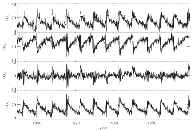
We have used for the present analysis the Greenwich sunspot group data during the period from 1874 to 1976, and the sunspot group data from the Solar Optical Observing Network (SOON) of the US Air Force (USAF)/ US National Oceanic and Atmospheric Administration (NOAA) during the period of from 1977 to 2009. The daily sunspot area and its latitude have been downloaded from the NASA website¹.

In Fig. 1 we show the averaged COL as a function of time during the period from 1874 to 2009. The COL is basically defined by

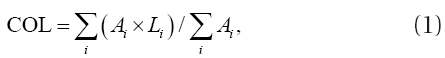
where A_i is the i-th sunspot’s area and L_i is its latitude. Thick and thin curves represent the yearly averaged COL and the monthly averaged COL, respectively. The summation is carried out over a calendar month or a calendar year, instead of the Carrington month. In the first and the second panels, we separately plot the averaged

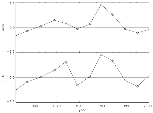
COL for sunspots appeared in the northern and southern hemispheres, respectively. Positive and negative COL represents the northern and southern latitudes, respectively. In the third panel, the averaged COL for sunspots appeared in both hemispheres is plotted. If the mean latitude where sunspots appear in both hemispheres is symmetrical, COL should be in a form of the random noise. However, we observe that the difference is large every time when the solar cycle begins. What is also barely seen is what is expected when there is a relative phase lag between the two wings. What we see is rather that the wings of the butterfly diagram is not symmetric, nor steadily drifts to the equator. In the last panel we plot the averaged COL of average of two hemispheres defined by

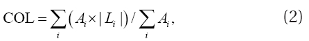
such that the absolute value of the latitude is used rather than the latitude itself. It is shown that the solar cycle begins when COL is high. And as the solar cycle proceeds COL decreases in general. We note, however, that COL is not monotonically decreasing as commonly assumed. Small humps (or short plateaus) between solar minima can be seen. Actually humps appear around every solar maxima.

1http://solarscience.msfc.nasa.gov/greenwch.shtml

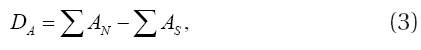
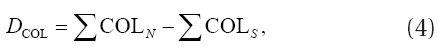
In Fig. 2, we show the difference between the north-

rern and southern hemispheres both in sunspot area and in COL. In the upper panel, we plot the difference in the sunspot area between the northern and southern hemispheres, which is averaged over the whole period for a given solar cycle. Therefore, the upper panel shows the asymmetrical behavior of the solar cycle and thereby which one is the dominant hemisphere. The difference is defined by

where Σ A_N and Σ A_S are thus the whole sunspot area appearing in the northern and southern hemispheres during a given solar cycle, respectively. In the lower panel, on the other hand, we plot the scaled difference of COL between the northern and southern hemispheres, which is also averaged over the period for a given solar cycle. The difference is defined by

where ΣCON_N and ΣCOL_S are the averaged COL in the northern and southern hemispheres during a given solar cycle as a whole, respectively. We note that COL is positive (negative), when the northern (southern) hemisphere is magnetically dominant. The exception occurs in the cycle 23.

Generally, there is no obvious reason why these two plots look similar, since the first panel tells us how large areas are covered by sunspots for a given hemisphere during the particular solar cycle while the second panel tells us the latitude where large sunspots are distributed for a given hemisphere during the particular solar cycle. For instance, supposed a bigger sunspot is at low latitude in the northern hemisphere and smaller sunspot is at high latitude in the southern hemisphere, it is not impossible that one can observe the positive D_A (northern dominance) and negative COL (southern dominance). Therefore, the fact that this kind of ‘odd’ thing does not happen for 11 solar cycles may give a clue that these two phenomena are regulated by a consistent mechanism.

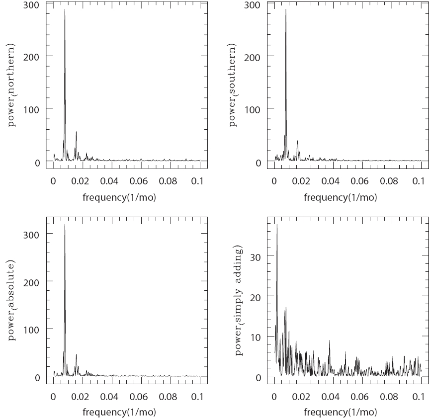
In Fig. 3, we show Lomb-Scargle periodograms (Press & Rybicki 1989) of COL in units of month^-1. The power shown here is in an arbitrary unit. In the upper left panel, we show the result of COL in the northern hemisphere. In the upper right one, we show the result of COL variation in the southern hemisphere. Not surprisingly, main peak corresponds to ~11 years. The secondary, yet significant, peak we also see here corresponds to ~5.5 years (confidence level is greater than 90%). We consider this period-

icity is due to humps between the minima we have seen in Fig. 1. In the lower left and right ones, we show results from COL of sunspots appeared in both hemispheres obtained by taking the unsigned COL, and the signed latitude into account, respectively. The power spectrum in the lower left panel is somewhat similar to power spectra in upper panels. In the lower right panel, one might expect a peak corresponding to ~ 9 year periodicity if s/he expects the solar North-South asymmetry (Chang 2007a, b). Instead, the periodicity of ~12 years (frequency ？0.007 month-1) can be found, which appears in the periodogram of the reciprocal of the total sunspot number,

(Ballester et al. 2005). This can be understood since we take the sunspot area as the weight function in COL calculations. It should be noted that the the highest peak corresponds to ~49 year periodicity (frequency ~0.0017 month^-1). It can also be understood in terms of a long term variation seen in Fig. 2. A similar periodicity of of ~44 years has been reported in the solar North-South asymmetry by Javaraiah (2003) and Zolotova & Ponyavin (2007), who suggested the existence of a '44-yr' cycle or 'double Hale cycle' and further ~80 year periodicity (Gleissberg 1971).

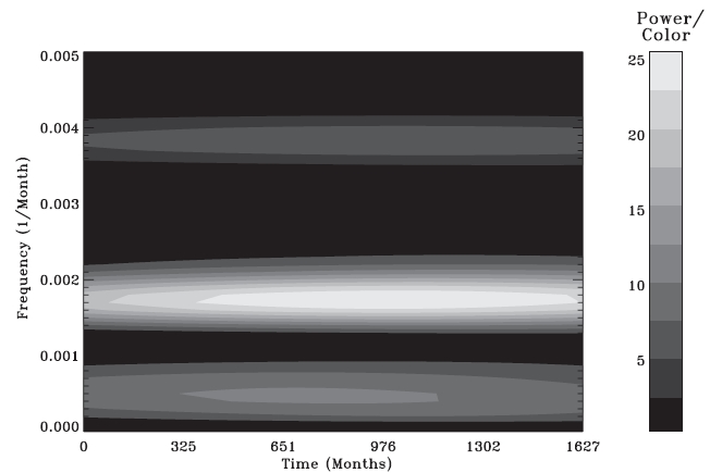
To see how its phase keeps consistently we analyze the same time series data using the wavelet transform technique (Chang 2006), which shows the power distribution in time. The power is normalized in terms of the mean level of noise so that the plot contains the signal-to-noise ratio by itself. As shown in Fig. 4, the power is apparently maintained for the almost entire period of data set. We have to conclude therefore that the oscillating component of ~49 year periodicity is significant and consistent. Moreover, one may also see another component with ~167 year periodicity (frequency ~0.0005 month^-1), which is also found in Javaraiah (2003) where the Sun’s motion about the center of mass of the solar system is related to the long term modulation in the differential solar rotation velocity derived by the sunspot observation.

Since the butterfly diagram is introduced to the field of solar study, the accepted paradigm has pretended that spots are scattered around a mean latitude, which monotonically drifts equatorward. For the sunspot activity a second order polynomial curve is widely used to give a fit to the monthly mean latitudes of sunspot activity. Accordingly, most of theoretical calculations have been aimed at developing models predicting the location of such a monotonic latitudinal migration of sunspots. On the other hands, some nonstandard solar magnetic models are introduced to describe non-steady equatorward progression (Bell 1960, Antalova & Gnevyshev 1983, Solanki et al. 2008).

We have examined the latitudinal variation of COL of sunspots in each hemisphere. As a fine structure of the butterfly diagram interests some researchers (Solanki et al. 2008, Ternullo 2010) an issue of how one may take care of different size sunspots will become more important. In this work we have suggested one way of doing this. By taking the area of sunspots into account, one may draw a more reliable conclusion on the evolution and distribution of sunspots, such as, 'active latitude' recently suggested. Another example of use of COL is a new diagnostic of the solar cycle and of models of the generation of the Sun’s magnetic field. As Solanki et al. (2008) demonstrated the latitudinal variation of position of sunspots can be used in distinguishing some dynamo models. On doing so, we may take care of the area of sunspots by using COL.

The summary of what we have found is as follows:(1) It is shown that the solar cycle begins when COL is high and that as the solar cycle proceeds COL decreases in general. COL in both hemispheres is not, however, monotonically decreasing as commonly pictured in theoretical calculations. Small humps (or short plateaus) between every solar minima can be seen around solar maxima.

(2) When the northern (southern) hemisphere is magnetically dominant, COL is positive (negative), except the solar cycle 23. The fact that this kind of ‘odd’ thing does not happen for 11 solar cycles may give a clue that these two phenomena are consistently regulated by a mechanism.(3) The periodicities of ~5.5 and ~11 years are found in each hemisphere. The periodicity of ~49 years are found in the power spectrum of the averaged COL. A possible periodicity of ~167 years is also noticed.