Surface topography measurement plays an important role in many applications in engineering and science. The threedimensional(3D) shapes of objects need to be measured accurately to ensure manufacturing quality. Optical methods have been used as metrological tools for a long time. They are non-contacting, nondestructive and highly accurate. In combination with computers and other electronic devices,they have become faster, more reliable, more convenient and more robust. Among these optical methods, interferometry has received much interest for its shape measurement of optical and non-optical surfaces. Information about the surface under test can be obtained from interference fringes which characterize the surface. Two- beam interference fringes have been used to investigate the shape of optical and non-optical surfaces for a long time [1]. The extracted phase from a single closed fringe pattern is ambiguous [2].This phase ambiguity can be easily removed by using the phase shifting technique [3]. The Fourier-transform method[4-6] can extract phase information very quickly, because it needs only a single interferogram to demodulate the unknown phase distribution. However, when an interferogram includes closed fringe patterns without a tilt i.e. without a carrier frequency, the Fourier transform method has difficulty in determining the complex fringe amplitude because the Fourier spectra of the interferogram cannot be separated completely.

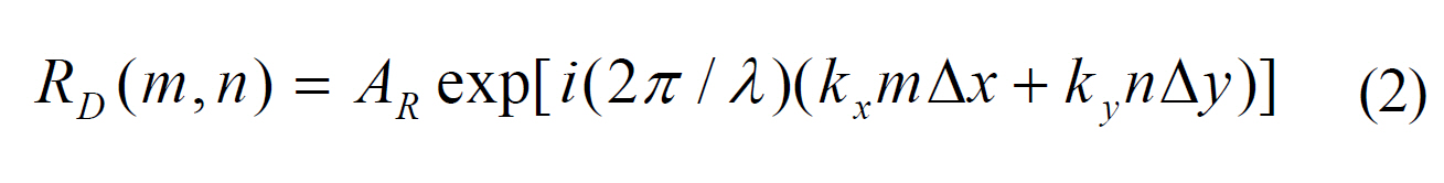
In this paper, the phase ambiguity from a single closed fringe pattern captured from the Fizeau interferometer was removed by using two algorithms. The first algorithm uses the off-axis geometry. In this algorithm, a single shot captured interferogram was processed numerically to reconstruct the surface object using computer programs [7-13]. The captured interferogram of the surface object was processed using Matlab codes to obtain the reconstructed object wave(amplitude and phase). The digital reference wave in the reconstruction algorithm should match as closely as possible the experimental reference wave. This was done in this paper by selecting the appropriate values for the two components of the wave vector k_x = 0.002955mm^-1 and k_y =0.01143mm^-1. The reconstructed phase map of the object surface was unwrapped and the unwrapped phase map was converted to height and the 3D reconstructed surface height was obtained. The second algorithm used the phase shifting technique. In this technique, four different interferograms of 0, π/2, π and 3π/2 radian phase shifts, respectively,were captured and corrected with the flat fielding method.

The demodulated phase map was obtained and unwrapped to remove the 2π ambiguity [14]. The unwrapped phase map was converted to height and the 3D surface height of the surface object was reconstructed. The reconstructed surface forms measured by the two algorithms were compared,and the results were in excellent agreement.

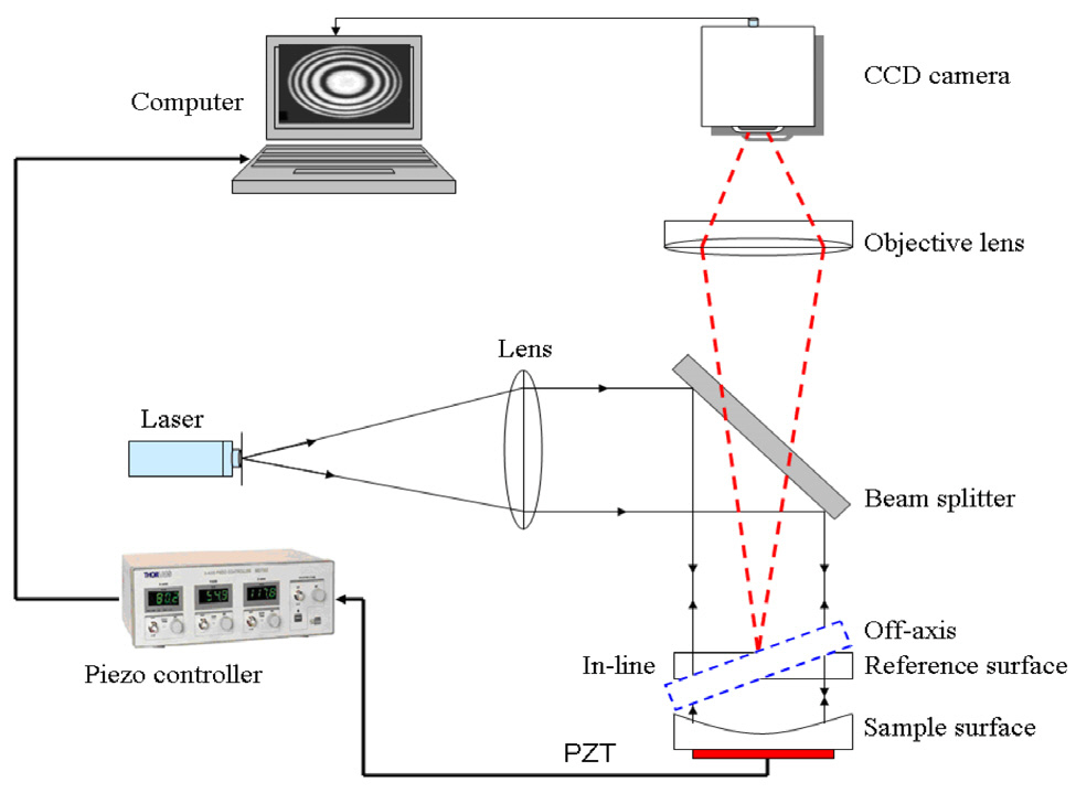
Figure 1 shows the schematic diagram of the optical setup of the Fizeau interferometer. The tested smooth spherical surface of 25.4 mm in size was mounted as an object in the interferometer. A laser diode beam passes through a collimating lens and expands. This expansion is necessary to illuminate a greater area of the surface to be imaged and to reduce the error measurement due to the inhomogeneity in the Gaussian beam. The collimated beam of the laser light falls upon the beam splitter, which transmits one half and reflects the other half of the incident light.The reflected collimated beam is then incident on the interferometer, which changes the path length of the light inside it due to the irregularities of the surface of the interferometer.

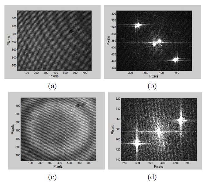
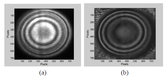
When the object and the reference (λ/20 flatness) are mounted close and parallel, two types of circular reflection fringes are seen; one, called the insensitive fringes, due to the interference from the two interfaces of the object surfaces,and the second, called the sensitive fringes, due to the interference of the reference interfaces and the object interfaces,. When 2D-FFT was applied for the inteferogram that had the two types of fringes (insensitive and sensitive)as shown in Fig. 2(a), six spectra were produced as shown in Fig. 2(b): three spectra produced from the insensitive fringes and the others produced from the sensitive fringes.In this case, the complex fringe amplitude becomes difficult to determine because the Fourier spectra of the interferogram

that contains the insensitive and the sensitive fringes are not separated completely. The problem of the insensitive fringes was solved by adjusting the object so that it became parallel to the reference (in-line scheme). Therefore,the insensitive circular reflection fringes were seen in the center of the field of view. These circular fringes were transformed to a background spectrum (DC term) when 2D-FFT was applied. By tilting the reference (off-axis case) as shown in Fig. 1, the sensitive circular reflection fringes were displaced, and nearly curved fringes at reflection with higher spatial frequency were seen, as shown in Fig.2(c). Only three spectra were obtained as shown in Fig.2(d) from Fig. 2(c) when 2D-FFT was implemented.

The interferogram was captured by the CCD camera of 1024×768 pixels with pixel size Δx=Δy=6.4μm. Assume that the coordinate system of the interferogram plane is the mn plane. When waves from both the object and reference of the interferometer meet to interfere, the intensity of the interferogram is given by:

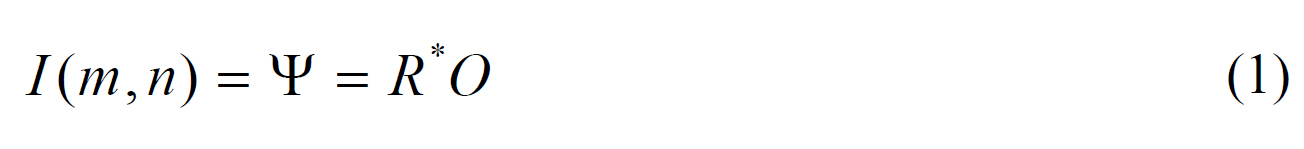
Here, Ψ represents the intensity of the recorded interferogram, O is the object beam, R is the reference beam,* denotes the complex conjugate and m, n are integers.The reconstructed wave front is an array of complex numbers. An amplitude-contrast image and a phase-contrast image can be obtained by using the following intensity[Re(Ψ )² + Im(Ψ )²] and the argument arctan {Re(Ψ )/Im(Ψ )},respectively. In the reconstruction process, the intensity of the interferogram is multiplied by the amplitude of the original reference wave called a digital reference wave (R_D(m, n)). If we assume that a perfect plane wave is used as the reference for interferogram recording, the computed replica of the reference wave R_D can be calculated as follows:

where, A_R is the amplitude, λ is the wavelength of the laser source, and k_x and k_y are the two components of the wave vector that must be adjusted such that the propagation direction of R_D matches as closely as possible with that of the experimental reference wave. By using this digital reference wave concept, we can obtain an object wave which is reconstructed in the central region of the observation plane. The captured interferogram of the surface object was processed using Matlab codes to obtain a reconstructed object wave(amplitude and phase). Figure 3 shows the flow chart of the algorithm that was used to analyze the off-axis interferogram.

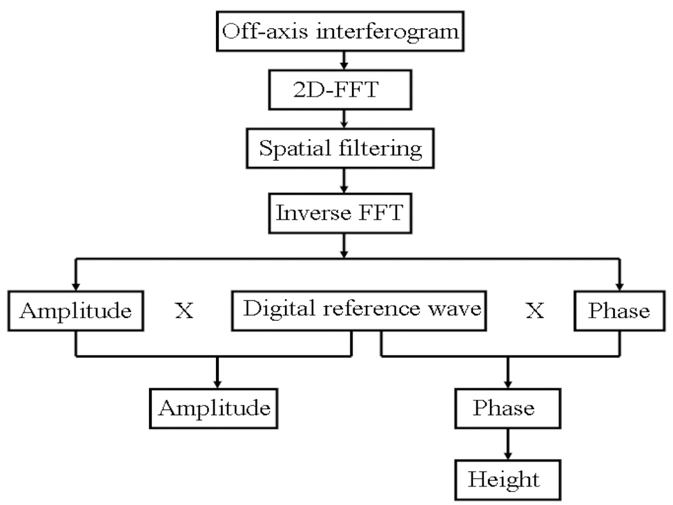
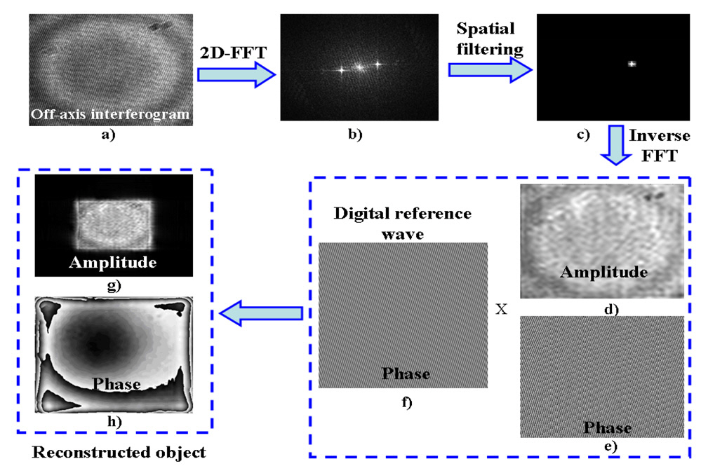
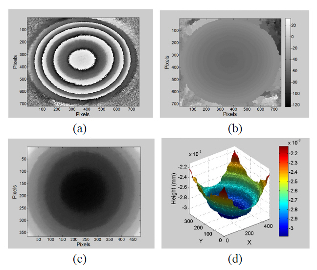
Figure 4 shows the detail numerical reconstruction process of a single shot off-axis hologram of a surface object. As depicted in Fig. 4(a) through 4(d), 2D-FFTs were implemented for the spatial filtering approach. The inverse 2D-FFT was applied after filtering out the undesired two terms, and the complex object wave depicted in Fig. 4(d)and 4(e) in the interferogram plane was extracted. After the spatial filtering step, the object wave in the interferogram plane was multiplied by the digital reference wave RD.The final reconstructed object wave (amplitude and phase)as demonstrated in Fig. 4(g) and 4(h) was recorded by selecting appropriate values for the two components of the wave vector k_x = 0.002955mm^-1 and k_y = 0.01143mm^-1.

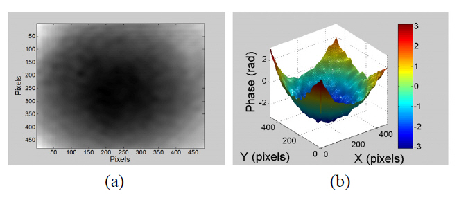
The reconstructed phase shown in Fig. 4(h) is non ambiguous and shows the results wrapped onto the range-π to π. In order to retrieve the continuous form of the phase map, an unwrapping step has to be added to the phase retrieval process [14].

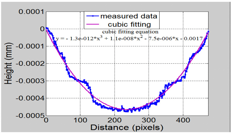
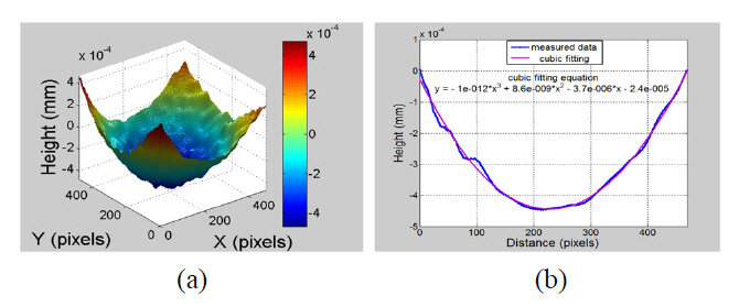
Figure 5(a) shows the 480×480 pixels unwrapped phase map for the wrapped phase map in Fig. 4(h). The 3D view of the unwrapped phase map is shown in Fig. 5(b).The phase information shown in Fig. 5(b) was converted to metrical 3D surface height information as shown in Fig.6(a). Figure 6(b) presents the measured profile curve along 480 pixels in the x-direction and its cubic fitting. The peak to valley value calculated from Fig. 6(b) was of the order of 0.45x10^-3 mm.

The smooth spherical surface has also been tested using four-frame phase shifting in-line interferometry. In the in-line case, the tested smooth spherical surface of 25.4 mm in size has been mounted as an object in the interferometer parallel to the reference as shown in Fig. 1. The interferogram was captured by the CCD camera of 1024×768 pixels. The CCD camera was calibrated by a process known as “Flat fielding” or “Shading correction” to remove the CCD camera offset and the inhomogenity of the Gaussian beam. Flat fielding can be illustrated by the following formula [15-16].

where I_c is the calibrated image; I_R is the non-calibrated object exposure; I_B is the bias or dark frame; M is the average pixel value of the corrected flat field frame; and I_F is the flat field frame.

Figure 7(a) shows the captured interferogram with the effect of the camera offset and the inhomogeneity of the collimated laser beam intensity, which were corrected using formula (3) in Fig. 7(b). The distance of the cavity between the object and the reference was changed very slightly by using a PZT varied by voltage. Four different interferograms of 0, π/2, π and 3π/2 radian phase shifts, respectively,were captured and corrected with the flat fielding method.The wrapped phase map from the corrected interferograms is shown in Fig. 8(a). The wrapped phase map is then unwrapped to remove the 2π ambiguity and the unwrapped phase map is shown in Fig. 8(b). Figure 8(c) shows 480 ×370 pixels unwrapped phase map at the middle of Fig.8(b). The phase information shown in Fig. 8(c) was converted to metrical 3D surface height information as shown in Fig.8(d).

Figure 9 presents the measured profile curve along 480 pixels in the x-direction and its cubic fitting. The peak to valley value calculated from Fig. 9 was of the order of 0.47x10^-3 mm.

As shown from the results and the cubic fitting equations,the measured value measured with off-axis geometry is very close to the value measured with the four-frame phase shifting technique, and the little deviation may be due to the vibration because the phase shifting algorithm is more sensitive to vibration than single shot off-axis geometry.

In interferometry, the path of the light has to be determined with high accuracy. The paths of the light rays can be determined accurately with elementary geometry and by successive applications of the law of refraction (or reflection);this method is known as ray tracing and is the most important current simulation method for macroscopic optical systems. The principle of ray tracing through refractive and reflective optical elements is well known [17-19]. The optical path length of a ray is calculated from the point of intersection of the ray with the surface of the plane of localization, where the rays meet to interfere. A ray tracing simulation program, which is written in the software“IDL”, traces the rays until they interfere and are detected.The program is written by applying the physical laws of reflection and transmission. The surface under test is characterized here in one dimension and is a straight line with a non zero inclination angle (Fizeau case). The intensities of the incident rays at transmission and at reflection are calculated using Fresnel coefficients. The amplitudes of the electric field that interfere at the first surface (in case of reflection) are squared to obtain the actual intensities,which constitute the fringes. When the rays are incident on the surfaces of the interferometer, some of the rays’intensity is transmitted and the remaining intensity is reflected. The total intensity of the reflected or transmitted rays is calculated by using the normal equation of Fizeau fringes

where A_n represents the amplitude vector of the n-th beam impinging on each pixel after 2n times of reflections.

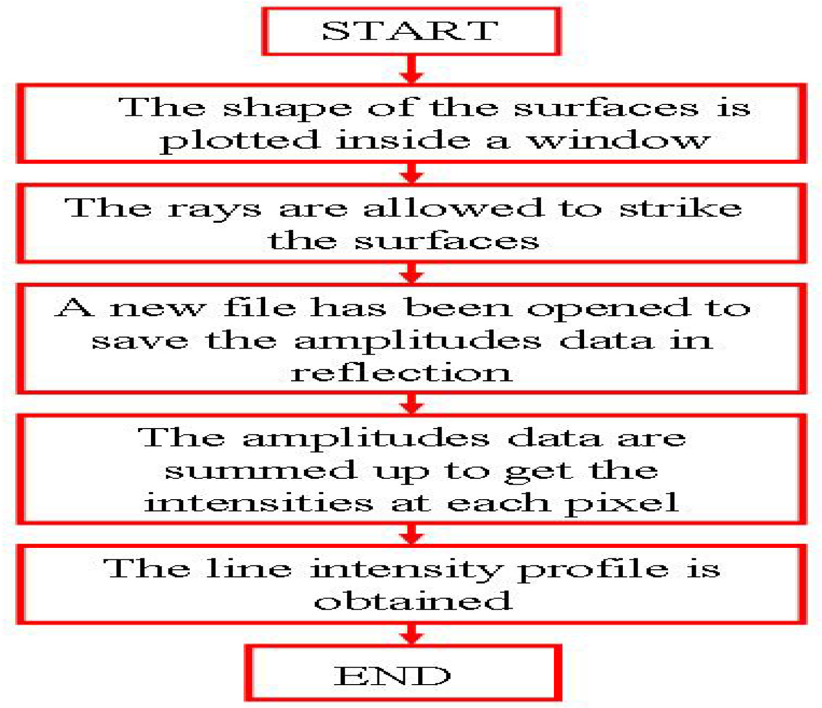
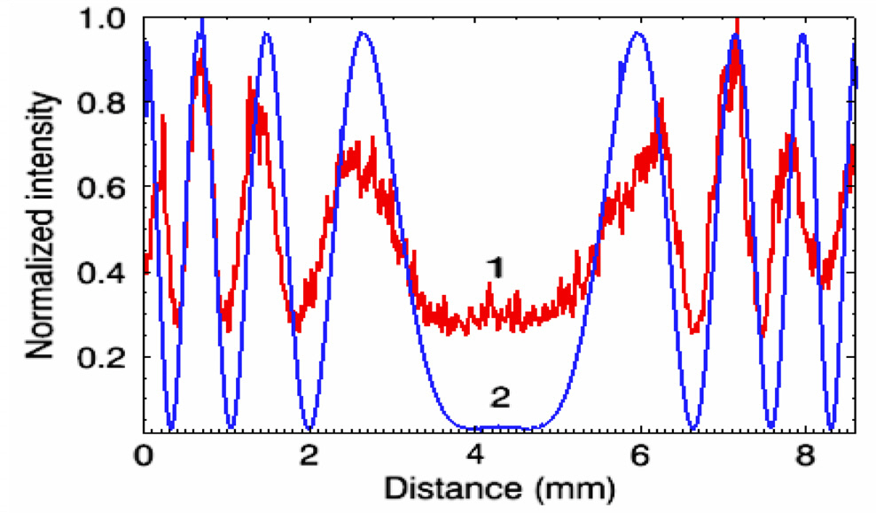
The value of the path difference changes directly with the slope of the surface. The path difference equals zero when the intensity is constant for highly parallel plate surfaces, but has a non-zero value if there is a small angle between the surfaces. The flowchart of the simulated interference fringes in reflection, produced with the ray tracing technique, is shown in Fig. 10. One-dimensional simulations of the surfaces (the reference and the object) are presented.Each simulated surface consists of two interfaces. The first two interfaces are for the reference that faces the incoming rays. The other two interfaces are for the object surface.Fig. 11 shows the simulation of the surfaces used that match the particular surfaces. The cavity distance was nearly 2 mm. This simulated cavity distance is very close to the experimental cavity distance.

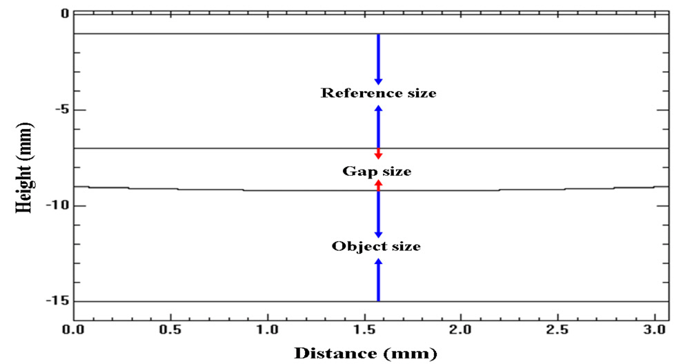
Figure 11 shows the in-line simulation fringes along 480 pixels. The reference and the object were 6 mm in size and the gap size was 2 mm. The conditions were taken in the simulation to match the practical conditions as well.The simulation fringes are cited here to estimate the uncertainty in measurement from the deviation of the simulation fringes and experimental fringes for this in-line case. Some sources of uncertainty in measurement were taken into consideration.Two important sources of error are vibration and air turbulence.These two sources can be estimated numerically from the deviation of the simulation fringes and experimental fringes as shown in Fig. 12. The deviation was estimated to be in the range of 5.0x10^-5 mm. The third source of uncertainty may be due to the nonlinearity of the voltage used in the experiment [20-21]. The standard deviation of the voltage from the mean was 0.025 V; this corresponds to a height of 1.0x10^-5 mm. Another source of uncertainity may be due to the incomplete parallelism of the incident beam and the uncertainty due to the incomplete parallelism was estimated to be in the range of 1.8x10-12 mm. In the in-line phase shifting scheme, the uncertainty budget [22] due to the factors considered was estimated to be of the order of 6.0x10^-5 mm.

For the single shot based off-axis interferometry, we can say that the main error sources would not be vibration and air turbulence but inevitable signal processing errors due to

the FFT based spatial filtering process. As well known, an energy leakage problem due to FFT process is inevitable in most applications. As a solution for this, the image processing technique called “apodization” can be used to reduce the fluctuation error due to the energy leakage problem[23]. And also, the spatial filtering process can increase the calculation error of the off-axis scheme since we can not filter only what we want from the spatial frequency domain data. According to what we estimated in the simulation code, the uncertainty of the off-axis scheme can be as small as around 1.0x10^-6 mm for a perfectly flat mirror surface in case that we apply the apodization filter for the off-axis interferogram. In this study, however, we have not applied this kind of technique. In that reason, the current uncertainty of the off-axis scheme can be estimated to be around 4.0x10^-5 mm.

Fizeau interferometer based on single shot off-axis geometry was used for measurement of a spherical smooth surface form. The results extracted from the single shot off-axis geometry were compared with the results extracted from the four-frame phase shifting in-line interferometry, and the results were in excellent agreement. The single shot algorithm is suitable for analyzing objects accurately and very rapidly. And also, the single shot algorithm is less sensitive to vibration and turbulence than is the phase shifting technique. Simulation has been conducted to estimate the uncertainty of the in-line and the off-axis scheme.