The GPS signal refractive index in the ionosphere varies according to frequencies. Thus, the dual frequency receiver capable of receiving both L1 and L2 frequencies can remove most of ionospheric errors through ionosphere-free combination (Hofmann-Wellenhof et al. 2008). However, the dual frequency receiver is relatively expensive, and thus if positioning does not require such observation accuracy as a few mm to a few cm, single frequency receivers are generally used. The single frequency receiver receives only L1 frequency, and uses the Klobuchar model, an ionospheric model designed for removing ionospheric errors.

The Klobuchar model can be used not only in removing ionospheric errors but also in modeling an ionospheric error environment. With the recent research on satellite navigation signal generation and processing, and the improvement of positioning performance, the need is increasing for GPS simulators designed for generating GPS signals. In order to generate highly reliable GPS signals for simulators, it is necessary to model a signal-receiving error environment more accurately. Of diverse error environments, the ionospheric error environment can be easily modeled using the Klobuchar model which has a simple structure and that makes calculation easy. To use the Klobuchar model, eight Klobuchar coefficients, namely, α_n,β_n (n = 1, 2, 3, 4), are needed, and Klobuchar coefficients are provided only through navigation messages (Klobuchar 1987). Thus, in order to model an ionospheric error environment for the generation of highly reliable GPS signals for simulators, the Klobuchar coefficient generation model is essential.

In this study, we developed a Klobuchar coefficient generation model and verified its accuracy. To develop the model, we used the broadcast (BRDC) navigation messages which include ephemerides of all the currently operating GPS satellites. We curve-fitted the tendency of three years of Klobuchar coefficients recorded in BRDC from 2006 to 2008, and developed the model. In this study, Klobuchar coefficients generated by the model and Klobuchar coefficients recorded in BRDC were defined as MODL coefficients and BRDC coefficients, respectively. Also, the Klobuchar model with the application of MODL coefficients and the Klobuchar model with the application of BRDC coefficients were defined as MODL and BRDC models, respectively. To examine the accuracy of MODL coefficients, the correlation coefficients between MODL coefficients and BRDC coefficients were determined. Also, the results of the MODL model and the BRDC model were compared with those of Global Ionospheric Maps (GIM), and the RMS error between these models was determined.

With the Klobuchar model, one can calculate total electron content (TEC) between the GPS satellite and the GPS receiver, estimate ionospheric errors, and remove total ionospheric errors by up to 50-60% depending on regions (Hwang et al. 2003, Komjathy 1997). To use the Klobuchar model, it is assumed that free electrons are concentrated in a hypothetical single layer with a thickness of 0 at the altitude of 350 km, the TEC is the highest at 2 pm local time, and the TEC is consistent at 9.24 TECU between 22:00 and 06:00 (Klobuchar 1987).

Input values necessary for the Klobuchar model consist of 3-D coordinates of the observation point and GPS satellite, observation time, and Klobuchar coefficients α_n and β_n (n = 1, 2, 3, 4). Klobuchar coefficients are designed to calculate the vertical delay and cycle, respectively (Seo 1994). Klobuchar coefficients, which are provided through navigation messages, are selected according to the two criteria as described in the following. The first criterion is observation date. The GPS master control station divides a year into 37 time segments, and set Klobuchar coefficient groups to respond to each time segment. The second criterion is the average solar flux for the previous five days including the relevant date. The solar flux is divided into ten classes, and Klobuchar coefficient groups are defined according to each class. By considering those two criteria, the GPS master control station has set 370 Klobuchar coefficient groups and, corresponding to observation dates and solar flux values, it decides which Klobuchar groups to use and provide it through satellite navigation messages (Seo 1994).

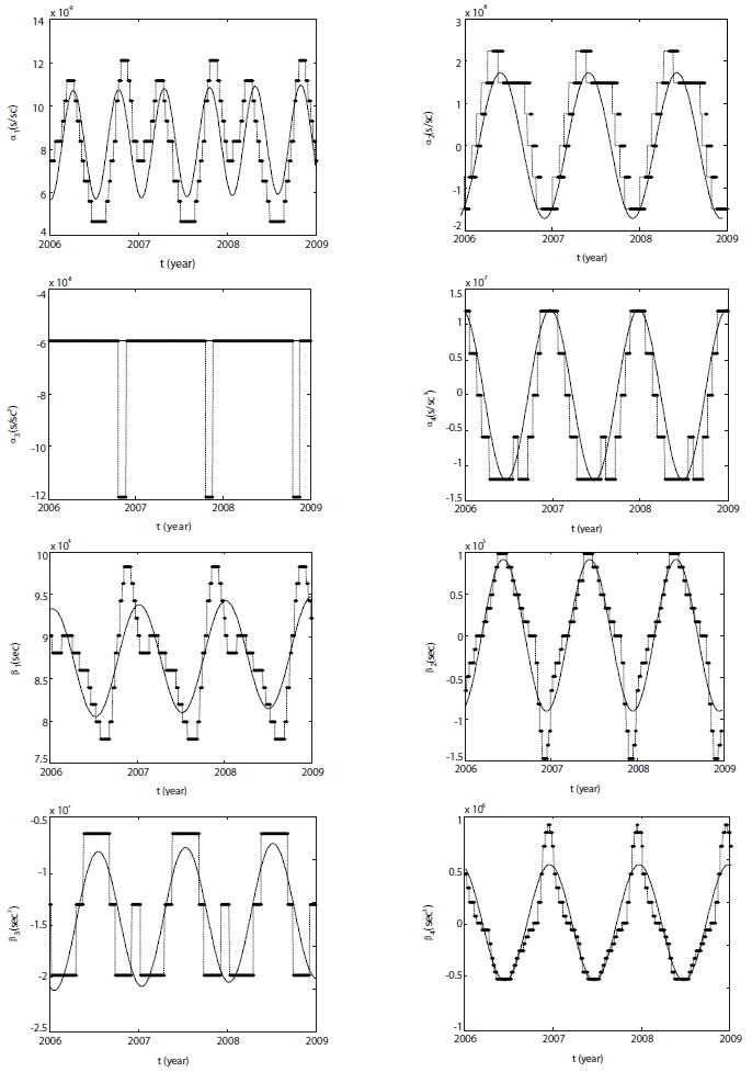
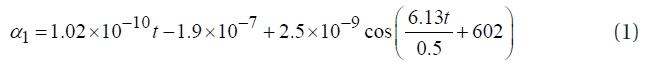
In this study, we analyzed the trends of BRDC coefficients inserted in navigation messages according to dates, and created a new model. BRDC navigation files between 2006 and 2008 that were provided by International GNSS Service (IGS) were used in creating the model. BRDC are navigation messages that include broadcast ephemerides with an interval of two hours for all the currently operating GPS satellites, and their headers contain BRDC coefficients for relevant dates. BRDC are created by day of year and can be provided from the IGS website, thereby making it easy to analyze changes in BRDC coefficients. In this study, eight types of BRDC coefficients were gathered, and their trends were analyzed according to dates. As a result, all coefficients except α₃ took a sinusoidal form. Thus, we curve-fitted each coefficient, and developed models with cosine and linear functions or constant and the result are shown in Eqs. (1) through (8). In each equation, t indicates observation date by year. In particular, α₁has semi-annual variations and α₃is a constant. All the other six MODL coefficients have annual signals in them.

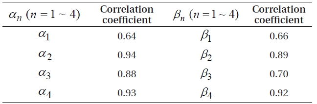
To evaluate the accuracy of the MODL coefficient generation model developed in this study, the correlation coefficients between the MODL and BRDC coefficients were computed, and they are shown in Table 1. As a result, correlation coefficients for α₂ and α₄ were high at 0.94 and 0.93, respectively, and those for α₁ and β₁ were relatively low at 0.64 and 0.66, respectively. In Fig. 1, α₁ and β₁, compared with other coefficients, show a great change in phase and amplitude, thereby presumably producing a low correlation with the cosine function-based generation model.

To verify the accuracy of the MODL coefficient generation model, we determined the vertical TEC (VTEC) above the Daejeon (DAEJ) observation station, and the period of analysis spans from January 1 to December 31, 2007. Likewise, to analyze the influences of the MODL and BRDC coefficients alone, we fixed observation time, and to determine the VTEC, we fixed the altitude angle between the GPS satellite and the DAEJ observation station, as 90°. Observation time is local time. And, the VTEC produced using the Klobuchar model was compared with that of GIM. The GIM model is produced by IGS Ionospheric Analysis Center, and provided in the IONosphere Exchange (IONEX) format, and it offers higher accuracy than the Klobuchar model (Choi 2009). The GIM model provides the global TEC values at grids of 2.5° by 5° resolution in terms of latitude and longitude. Thus, the results of the MODL model and the BRDC model were compared with the values of the GIM model for latitude 35° and longitude 125° which is closest to the DAEJ observation station located at latitude 36.399° and longitude 127.374°.

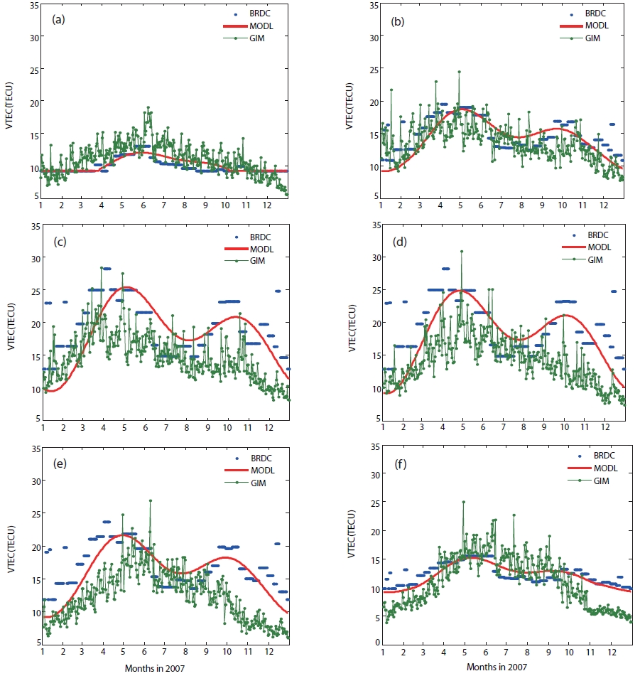
Fig. 2 shows the daily VTEC of the BRDC and MODL models produced using the observation time fixed at the interval of two hours, namely, 09:00, 11:00, …, 19:00. In Fig. 2, the blue dot and the red line each show the VTEC of the BRDC model and the MODL model, and the green line indicates the values of the GIM model. As shown in Fig. 2, the VTEC of the BRDC model and the VTEC of the MODL model had a similar size and trend, and they were larger in spring and autumn than in summer and winter. This result is consistent with the generally known TEC trends according to seasons. The TEC values of each model vary according to observation time, and they are the highest at 15:00. And, generally, the VTEC values of the GIM model fluctuate significantly by dates, compared with those of the BRDC and MODL models. In Fig. (a), the VTEC of the Klobuchar model has a constant value from early October through the end of March because the interim values of the equation as calculated did not meet the conditional expression of the Klobuchar model since the angle of elevation and the observation time which were the input values required for the Klobuchar model calculation were fixed.

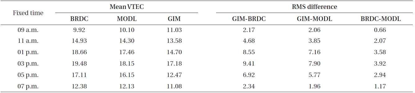
Using the results of Fig. 2, the average VTEC of the three models and the difference between them were analyzed. Table 2 shows, according to observation time, the average VTEC of the three models, and the RMS difference between them. The average VTEC, according to observation time, was the lowest at 09:00 and the largest at 15:00 for all of the three models. In the case of the Klobuchar model, the average VTEC of the BRDC model and the MODL model was 19.48 TECU and 18.15 TECU, respectively, at 15:00. In the case of the GIM model, the average VTEC was 17.18 TECU at 15:00, showing the smallest value among the three models. For the average VTEC values by model, the BRDC model had the largest value, and the GIM model had the smallest one.

The RMS difference calculated between models is given below. The RMS difference had the minimum value and the maximum value at 09:00 and 15:00, respectively. Compared with the GIM model, the RMS difference of the BRDC model and the MODL model was calculated as 9.41 TECU and 7.90 TECU, respectively. The RMS difference between the GIM model and the Klobuchar model was created presumably partly because the geographical coordinates of the GIM data were inconsistent with those of the DAEJ observation station. The RMS difference between the BRDC model and the MODL model was 3.92 TECU, and this difference, converted into the distance error, is 0.63 m. Considering the required accuracy of an GPS simulator by the users of single frequency receivers, a difference of 0.63 m can be regarded as negligible. Thus, it is deemed that the MODL coefficient generation model developed in this study can be used in modeling the general ionospheric error environment for GPS simulators.

In this study, we analyzed the trends of BRDC coefficients provided by three years of BRDC files from 2006 to 2008, and developed the MODL coefficient generation model for simulators. The correlation coefficient between the MODL coefficients and BRDC coefficients was the highest at 0.94 for α₂, and the lowest at 0.64 for α₁. To validate the accuracy of the MODL coefficient generation model, we assigned MODL coefficients and BRDC coefficients to the Klobuchar model and calculated VTEC, and compared the result with the GIM model. As a result, compared with the GIM model, the RMS difference of the BRDC model and the MODL model were calculated as 9.41 TECU and 7.90 TECU, respectively. The RMS difference between the results calculated through the MODL model and the BRDC model was 3.92 TECU. Given the assumption that a GNSS simulator does not need to produce ionosphere errors at an extreme accuracy, 3.92 TECU is deemed no problem. In this study, only VTEC was analyzed, but with GPS simulators, slant TEC along the line of sight is also needed; thus, future studies should conduct a comparative analysis of slant TEC. Also, in this study, the model was developed using only BRDC coefficients for the period corresponding to the solar minimum; thus future studies should use BRDC coefficients for the eleven-year period which all covers the solar maximum and minimum.