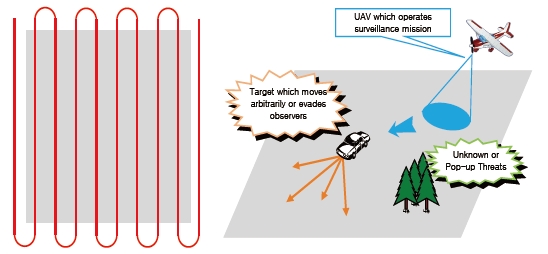
A surveillance mission is operated to monitor or observe regions of interest, and CCTVs or robots collect whatever information available from the site. On the other hand, a reconnaissance mission is a mission used to gather specific information of certain interest to an operator. Thus, intelligence, surveillance, and reconnaissance (ISR) become very important when protecting ally forces and reducing damages by enabling missions to destroy essential facilities or threats. Since there are currently no major enemies, decision-makers should collect as much information as possible for protection missions. An exhaustive coverage path-planning, as shown in the left figure of Fig. 1, is widely used in surveillance missions. It is very powerful when there are no threats, since an unmanned aerial vehicle (UAV) may obtain information from a whole map without an empty zone. Some studies using such a path-planning approach under obstacles have already been published (Moon and Shim, 2009). However, this approach is ineffective for situations in which targets are capable of recognizing observers and subsequently avoiding those observers as a result of the recognition. If the observers' paths are simple and easily predictable, then targets will attempt to hide or evade their observers. Thus, the observers could not achieve a goal. Sometimes optimal paths are planned off-line. However pre-defined paths cannot be updated in real-time; therefore, the paths may not accomplish the goal in dynamic environments.

A search mission is very similar to surveillance for cases in which a mission is needed to verify whether some problems occur or not in the regions of interest. For example, assume that a mission is operated in a prison to watch the prisoners. The mission should assume that there are some convicts, and observers should carefully watch locations where convicts can easily hide. If observers move on the simple exhaustive coverage paths, then convicts will predict their movements well and hide somewhere. This is the reason why exhaustive coverage path-planning, such as lawn mowers, cannot exhibit satisfactory performance in a surveillance mission.

A large amount of research about search missions has been conducted such as optimal search theory and exhaustive geographic search (Spires and Goldsmith, 1998; Stone, 1975). Yang et al. (2002a, b, 2004), Sujit and Ghose (2003, 2004a, b), Polycarpou et al. (2001), Flint et al. (2002a, b), and Bertuccelli and How (2005) presented major progress with the solution of a search mission problem. Polycarpou et al. (2001) proposed a basic framework for a cooperative search. Vehicles are under some assumptions such as (i) a limited target sensing capability, (ii) a limited wireless communication, and (iii) self computations to make online guidance. Bertuccelli and How (2005) introduced the beta distribution to compute target existence probability. They applied the algorithm to both stationary and moving target problems (Bertuccelli and How, 2005; 2006). The aforementioned research assumes that the world is ideal and simple. This assumption simplifies a problem and allows for the construction of a basic framework. However, this assumption is subject to limitations when algorithms are applied on small UAVs or real scenarios.

This paper focuses on a simple and realistic algorithm that possesses the flexibility to be easily handled by operators under dynamic environments, and can be loaded in smallsized UAVs. This paper consists of several sections. First, a problem is formulated by defining information shared among cooperative UAVs. Then an environment, such as mission fields, and an information point (IP), which quantifies certainties of the mission fields are defined. Next, cost functions for the main algorithm are defined. The algorithm is named waypoint planning algorithm using cost functions for surveillance (WAPACS). WAPACS offers waypoints over which UAVs will fly to collect necessary information. To generate a preliminary path to the waypoint, A* algorithm is introduced, and it selects sub-waypoints from a starting position to the waypoint. A* algorithm used in this paper is modified to generate the shortest path as well as a way to achieve better surveillance performance. This means that it is a trade-off between the shortest path and the path to acquiring more information.

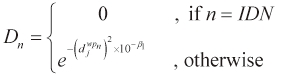
Cooperative operation entails information sharing between two or more UAVs. Each UAV is a decentralized decision-maker; therefore, WAPACS operates on each UAV individually. It is difficult to share and store obtained information because the amount of information is generally very large. Wireless communication is not robust and has a limited bandwidth; additionally, storage devices are useless since information stored in UAVs cannot be used by operators. Therefore, it is assumed that all information is transmitted to an operator unilaterally: each UAV shares a little information and decides its own waypoints using WAPACS. Information shared by each UAV consists of current position, current waypoints and the UAV identification numbers (IDN). Each UAV possesses a specific and unique IDN; in other words, IDNs are not duplicated. The use of this information enables operators to estimate certainties of mission fields. Furthermore, positions, waypoints, and certainties are used by WAPACS when the system selects the next waypoint. This will be explained further in the section of cost functions.

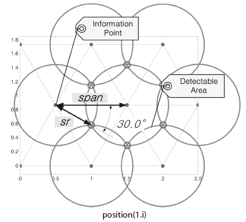
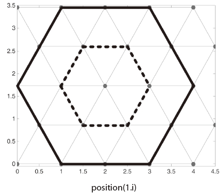
A grid or cell map is typically used for representing an observed field, and to simplify it (Bertuccelli and How, 2005; Flint et al., 2002a, b; Sujit and Ghose, 2003; Yang et al., 2004). Mathematical forms of the algorithms are simplified with the reduction of computation time due to such assumptions or modelings. For this study, IPs are spread in mission fields in the form of hexagonal grids, as shown in Fig. 2; however, rectangular grids are used in a study conducted by Lim and Bang (2009). These points are defined IPs because certainty is stored at each IP, and certainty quantifies the amount of information on an IP. Each IP represents its surroundings. If certainty is sufficiently high, then monitoring around the IP area is no longer required.

However, the use of IPs spread in mission fields as described does not imply the assumption that the world is made of discrete domains. UAVs fly over continuous domains in which IPs represent each section of the observed fields. This is a major difference from research mentioned above. In Yang et al.'s (2002a, b, 2004) and Sujit et al.'s (2004a, b) research, UAVs can only move on a grid or cell at each time step. A mathematical optimal solution can be derived when vehicles can only move on a grid or cell based on the assumptions; however, the simulation results will be much different compared to actual situations. The object of this research is not to derive a mathematical optimal solution, but to propose an efficient method which can be used in real scenarios; therefore, it is best to use real 2-dimensional x, y coordinates for positioning UAVs.

The interval between each IP should be considered. Small intervals indicate closely positioned IPs. Thus, the algorithm requires more computational power, and they describe real world well. On the other hand, if the interval is large and the IPs are correspondingly distributed over a broad range, less computational power is required; however, the information obtained under this arrangement is not sufficient to monitor whole fields. Therefore, a reasonable interval should be defined depending upon the performance of sensors. We assume that sensors equipped on UAVs monitor the area around the UAVs, and they have a limited distance when detecting targets, sr. Therefore, operators can receive information from a circle area, for which the center is an UAV position. Using this performance limitation, the maximum available interval can be defined as

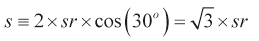
to minimize duplicated detection areas and to eliminate empty spaces.

The amount of information acquired from each IP is quantified into certainty, c, for which the maximum value is equal to unity. The maximum value signifies that operators have complete knowledge. A minimum value of zero indicates that there is no available information. Certainty increases when an observation is made in the area of interest. However, certainty decreases over time if an observation is not made. An update rule can be expressed as

where d_{i j} is a distance from the ith UAV to the jth IP and c'_(xj,yj) is the certainty of the j^th IP at time t. If certainty is updated with τ₁ = 0.99 and τ₂ = 0.9 at every second, the certainty level is decreases to 50% from the original level after about 69 seconds when monitoring is not performed (Lim and Bang, 2009).

In this section, an algorithm named WAPACS is introduced. The algorithm uses various cost functions based on, but not limited to, certainty, distance, and level of interest. WAPACS provides a next waypoint for an UAV which implies what should be observed. Therefore, it may select a point with the lowest certainty in the map. However, simply selecting the point is not useful and intelligent; hence, the algorithm considers various circumstances such as the elements mentioned above, and selects a point with the lowest cost. Consequently, WAPACS improves surveillance performance in a cooperative mission. The following sections will explain each cost function in detail.

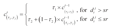
In surveillance missions, information about field states is highly important. Such information includes terrain, threat positions or positions where targets can easily hide. Information is stored at each IP, and certainty shows the amount of information. It increases when an observation is made in the area of interest. However, certainty decreases over time if an observation is not made. Eq. (2) can be used to compute cost. However, there exists a discrepancy which cannot be overlooked. The point with the lowest certainty has the lowest cost; therefore, the algorithm selects that point, considering that single IP independent of the other IPs. However, observing other points with a slightly higher certainty could be more efficient when the point is surrounded by points possessing high certainty. In other words, selecting that single point can be inefficient since it is required to pass through the surrounding points with higher certainty in order to observe the single IP. By observing a single point, the goal of monitoring a wide area may not be achieved. Therefore, it is suggested that each IP contains the average certainty of neighboring IPs, as is shown below (Lim and Bang, 2009).

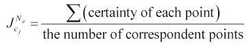
Fig. 3 describes Eq. (3) sufficiently well. If N_a = 0, then the cost becomes certainty only of it. Moreover, if N_a = 2, then the cost becomes the average certainty of 19 points. Undoubtedly, IPs located outside the fields and within areas outside the scope of interest should be neglected when certainty is averaged. The maximum value of this cost is equal to 1, while the minimum is 0.

In this research, a cooperative operation is considered. Each observer has a same algorithm and information such as cost functions. Hence, it is possible to select a close point, or even the same point, as their waypoints. This situation is very inefficient since monitored areas of them will be overlapped each other. Therefore, a cost function should consider waypoints of each observer as below (Lim and Bang, 2009).

where

and N_u stands for the number of total UAVs, β₁ > 0 , and d_j^wPn is a distance from the jth IP to the waypoints of nth UAV. The first line of Eq. (4) implies that its previous waypoint is neglected when the cost is computed since this cost function is related to waypoints of co-workers. Using β₁ an operator can adjust the cost curve with respect to distance. If β₁ is sufficiently small, then the cost quickly converges to zero. The maximum cost is also equal to 1, and the minimum is 0. This is the first key point explaining why this algorithm can be used in cooperative surveillance mission.

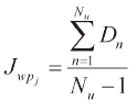
WAPACS is the algorithm for cooperative operation using multiple observers. Therefore, it will be better that each observer should be assigned an observation area separate from the other observers. Thus, the overlapping of monitored areas will be reduced. However, if the given sectors are fixed, the algorithm will give targets more opportunities to avoiding the observers since targets find it sufficient to consider only a single observer. That is, observation areas should occasionally be re-allocated after long periods of observation. Hence, another cost function is defined as (Lim and Bang, 2009)

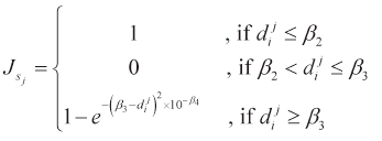
where β₃ > β₂ >0, β₄ > 0, and d_{i j} is a distance from the ith UAV to the jth IP. The cost reaches its maximum from a current position to points within β₂ (m). And, the cost is minimum for the points located within β₃ (m) and outside β₂ (m). Using β₄ , an operator can adjust the cost curve with respect to distance. If β4 is sufficiently small, then the cost converges to zero very quickly. The first equation yields the maximum cost. Since aggressive maneuvers are required to follow the points, observing targets becomes difficult, subsequently requiring more kinematic or potential energy. A cost of points outside β₃ (m) becomes large than the minimum.

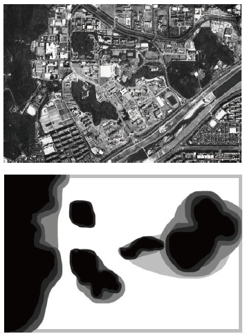
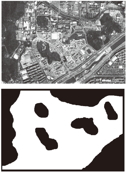
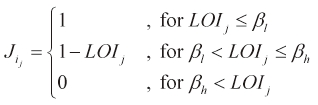
All areas do not have the same level of interest. Some areas have higher levels interest, while some areas are deemed unnecessary to observe. This information is passed along to operators. For example, in Fig. 4 black areas imply that no observation is needed, and white ones imply high levels of interest by an operator. Gray areas indicate a lower priority of observation than the white areas. Thus, cost can be defined as

where LOI, is a level of interest of the j^th IP, β _l is low threshold, and β_h is high threshold. This intuitive equation could be used for other purposes such as avoiding threats. If an operator assigns a value of zero to an area containing threats with, WAPACS will then provide a maximum cost. Consequently, the points in that area will not be selected.

After selecting the next waypoint, the well-known A* algorithm is used to generate preliminary paths. To generate it, the A* algorithm selects sub-waypoints from the current position to the waypoint. Sub-waypoints are the points which draw the preliminary path from a starting point to a final waypoint. UAVs approach the waypoint by passing through many sub-waypoints. That is, the sub-waypoints of each UAV will be observed soon by someone. Therefore it is more efficient that ignoring those sub-waypoints as next waypoints even if the points have the lowest cost. This is the second key point justifying why this algorithm can be used in a cooperative surveillance mission. Each path of UAV will not be duplicated due to this constraint.

Using the aforementioned cost functions, the final cost is computed for each IP. In this procedure, the concept of the weighting factor is introduced to adjust the priority of each cost function.

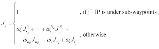
where

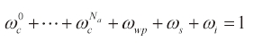
Each weighting factor determines the priority of each cost function. For example, if ω_c ⁰ is 1 and the others are 0, the algorithm will try to visit every IP in the case of the fixed certainty update rule without Eq. (2). If ω_wp is 1 and the others are 0, then the algorithm will try to disperse UAVs and they will spin around at the corners of a map. If ω_s is 1 and the others are 0, then UAVs will try to visit close areas and wander in a map. And if ω_i is 1 and the others are 0, then they want to visit areas with high level of interest only.

As mentioned before, the points under sub-waypoints of co-workers will have the maximum cost to avoid being selected as a final waypoint. If there are candidates of subwaypoints with the same cost, then the algorithm selects the closest point to the decision maker.

After selecting a final waypoint using various cost functions, A* algorithm generates a preliminary path by selecting the subwaypoints. Details of the A* algorithm have been published in the reference, Artificial Intelligence, by Russell and Norvig (2003). Typically, a starting node is taken as the starting point; however a position of an UAV cannot be used directly as the starting node since it is not always on IPs. Therefore the closest IP from the UAV is considered the starting node, even if the UAV is outside map. A goal node is a terminal point of the preliminary path. Additionally, it is the waypoint selected using the various cost functions described in this paper.

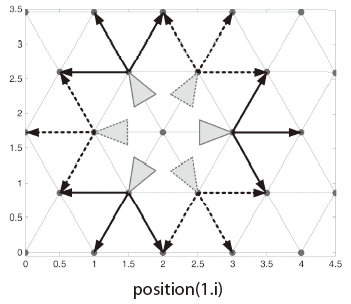
A successor function returns possible children nodes from a certain node. It will return all surrounding nodes if it does not consider a dynamic restriction of UAVs. Observers used in this algorithm are UAVs; therefore, there exists a clear dynamic restriction on heading rate. Aerial vehicles, with the exception of helicopters, cannot change headings in standing. Therefore, a parent node should be input in the successor function. The successor function will then return nodes which generate a straight or diagonal path, as shown in Fig. 5. That is, it means that opposite directional paths will not be generated by this successor function.

The heading restriction is not the only issue children nodes are returned. Nodes located outside the map are, undoubtedly, not returned. Additionally, nodes are not returned if the level of interest is lower than β _l ; in which case, observations of the nodes fitting this criteria are deemed unnecessary.

Summation of each action cost is the path cost of a current node. The path cost signifies the cost required when an object moves from a starting node to a current node. Aerial vehicles require more energy when they turn. That is, the cost of a diagonal action is greater than that of a straight one. The certainty and a level of interest are included in the path cost. Consequently, the path cost is defined as

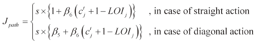
where s is the interval between each IP defined in Eq. (1), and β₅ and β₆ are greater than one and zero, respectively. Due to β₅ , a path cost will increase when a path is bent., An operator can adjust the cost function for obtaining an optimal path using β₆ . If β6 is zero, then a path will be the shortest path; and if it is sufficiently large, then the path will pass through an area of a low level of interest. This means that it is a trade-off between the shortest path and the path to acquiring more information. If certainty is high, then the cost increase; if the level of interest is high, then the cost decreases.

A heuristic function should be admissible in order to make the A* algorithm stable (Russell and Norvig, 2003). An admissible heuristic function should return a smaller cost than the real cost in order to reach the goal node. If a distance is set as the heuristic function, it is admissible, since the path cost cannot be larger than the distance for a path cost defined with Eq. (9).

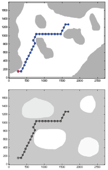
An example is introduced in Fig. 6. Waypoints, including the final waypoint and sub-waypoints, are represented with the level of interest in the left figure. Black regions designate areas of little to no interest, therefore, A* selects points avoiding those regions. The background of the figure on the right represents certainty. The certainty of white regions is equal to 1, hence A* selects points avoiding them.

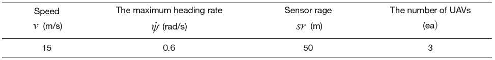
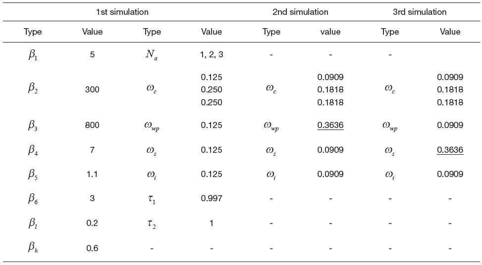
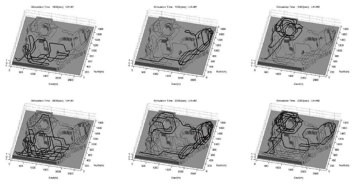
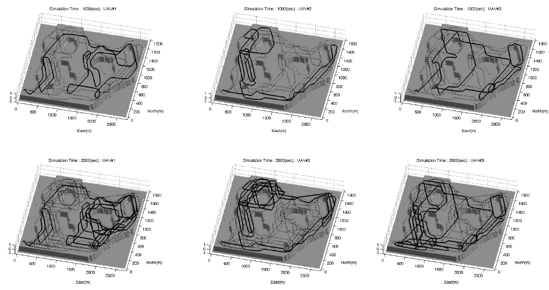
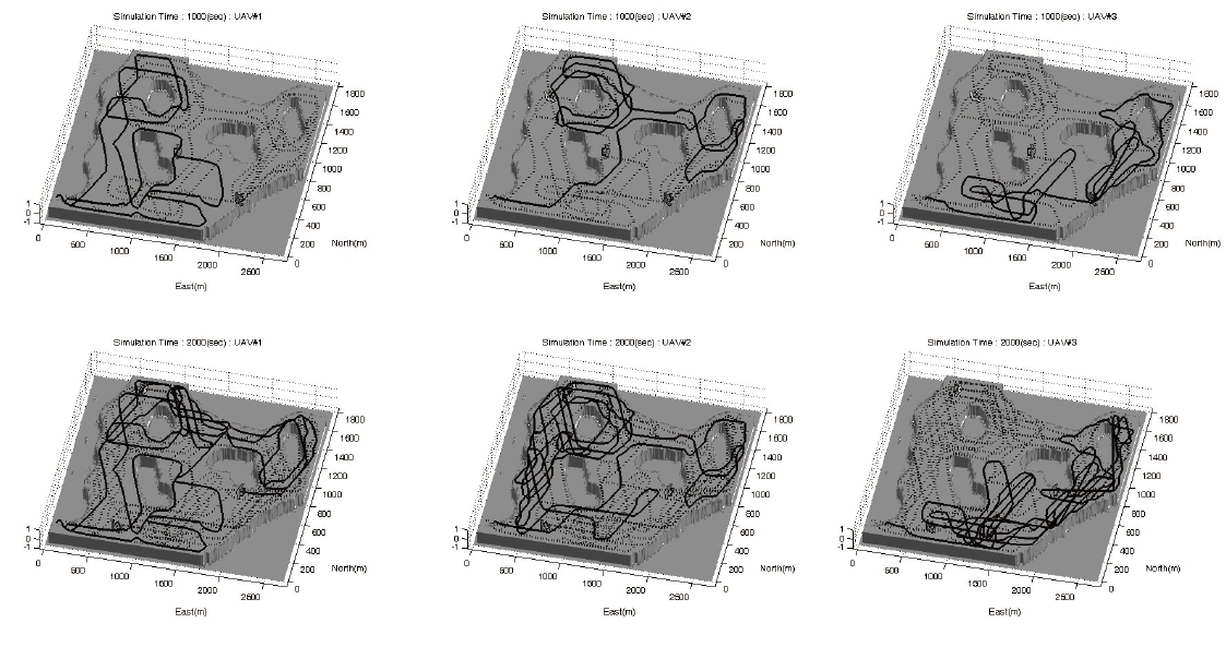
Simulation results based on the actual map of an area under surveillance are elaborated in this section as you can see in Figs. 8-10. The performances of UAVs are presented in Table 1, and the level of interest is shown in Fig. 7. The key parameters are shown in Table 2. One can understand the effects due to ω_wp and ω_s through 2nd and 3rd simulations, respectively. A typical waypoint guidance law is used in these simulations.

The weighting for the cost about a distance from the waypoints of co-workers becomes larger in the 2nd simulation. Consequently, they fly separately in far spaces. If the weighting for a distance from these waypoints becomes larger, then they do not observe a near area, then they turn around the whole map.

The simulation results illustrate the desired performance of the proposed WAPACS algorithm for a surveillance mission. Three UAVs fly over the whole map, and observe the areas with exception to those areas in which observation is unnecessary. The paths are not readily estimated; therefore, observation by the UAVs is impossible to avoid by estimating the paths even if the targets are equipped with intelligence. The three UAVs are allocated separate areas to avoid duplicated tasks and enhance cooperation among the UAVs. Moreover, if the UAVs occasionally exchange areas, targets will have a difficult time recognizing the paths of the UAVs. Finally the proposed algorithm requires less computational power; therefore, one can envision implementing them in small-sized UAVs.