Terrain referenced navigation (TRN) estimates an aircraft status, by using a radar altimeter to measure distance between terrain and the aircraft. TRN has been widely investigated since the 1980s [1-5], and it is usually integrated with an inertial navigation system (INS), to prevent drift error. The integration scheme is similar to the well-known GPS/ INS navigation. TRN compensates for drift, and provides a bounded navigation solution.
Filtering methods, such as a Kalman filter (KF), can be applied to TRN. However, because of the nonlinearity of the measurement equation, the KF cannot be used directly. Alternatively, an extended KF (EKF) linearizing measurement equation could be adopted. The linearized equation requires terrain slope calculation, for which the slope could be estimated, using the terrain map. When the position error between true and estimated positions is small, the estimated slope would be accurate; however, because of terrain nonlinearity, the accuracy may degrade as the position error increases. Because the Jacobian matrix of measurement equations in the EKF consists of the terrain slope, inaccuracy of the slope estimation could break the filter consistency. In other words, conventional EKF may no longer be valid, with large position error covariance. To overcome such a problem, various strategies have been employed in TRN, such as a bank of KFs [1], a particle filter [2], and an unscented KF [3].
In addition, Hostetler and Anderas [4] proposed the slope estimation method, using the least squares in EKF-based TRN. The method searches the best slope, in the least squares sense, representing the terrain map over the linearization region determined by the position error covariance. Reference [5] utilizes linear regression, composed by two least squares at latitude and longitude axes, respectively. In this paper, two slope estimation methods modifying the previous method [5] are proposed. One is planar regression, estimating the slope using a plane, instead of the two lines of the previous linear regression. The method could incorporate correlation of the two axes, so the slopes could be more accurate than the previous one. The other method is weighted planar regression. By considering that the state is estimated using a Gaussian probability density function (pdf) in a KF, additional weights formed by the Gaussian pdf are multiplied to the proposed planar regression. Two Monte Carlo simulations are performed, to compare the performance between the previous and two proposed methods, by considering the filter divergence probability and convergence speed.
This paper is summarized as follows. Strapdown INS kinematics and EKF-based TRN are introduced in Section 2. In Section 3, the previous and two proposed slope estimation methods are discussed. Monte Carlo simulations are conducted to compare performances between the three methods in Section 4, and a conclusion is given in Section 5.
2. Extended Kalman Filter Formulation
Strapdown INS kinematics are adopted to propagate aircraft status. An error-state is propagated, instead of the full-state, and the kinematic equations are described as

The error-state
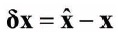
is the difference between the estimated state

and true state x.
The term
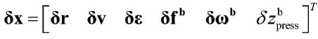
is composed of of errors of position, velocity, Euler angle, IMU biases and barometer bias. w is a noise vector depending on the IMU specification, and components of
Measurements equations expressing the sensor outputs of radar altimeter and pressure altimeter are such that
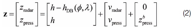
where,
are sensor outputs, random noise and bias terms, respectively.

as
where,
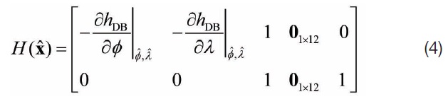
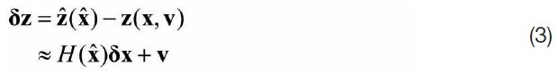
Now, the error-state EKF can be directly formulated using kinematic equations, measurement equations and Jacobian matrices
3. Terrain Slope Estimation Methods
The Jacobian matrices in Eqs. (1) and (4) are statedependent, and this may cause filter divergence. In TRN in general, nonlinearity is more profound in measurement equation, than in kinematics. Jacobian
In conventional EKF, terrain slopes are estimated by taking partial derivatives along the latitude and longitude at the estimated position

This method is valid when

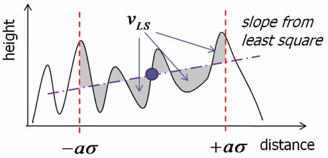
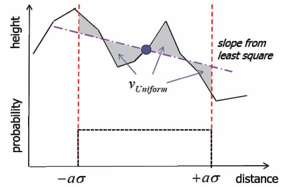
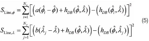
however, estimation accuracy decreases as the position error becomes larger. To remedy such a problem, stochastic linearization (SL) is suggested in [4]. SL utilizes the least squares method to obtain the slopes. Fig. 1 depicts the method. In [5], two linear regressions are performed to obtain the slopes.
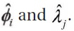
where,
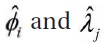
denote each position in the estimated region, and their mean position is represented by
Terrain
slopes are defined by
The variance of residual error shown in Fig. 1 can be given by
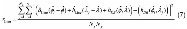
which is added to the sensor noise covariance, to incorporate the linearization error of slope estimation.
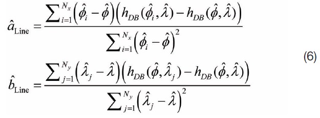
In previous research [5], two linear regressions are applied, to derive terrain slopes at each axis. One axis is fixed, while the slope of the other axis is computed. For example, longitude is fixed at the mean position

when latitude slope
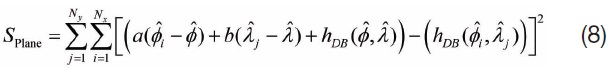
The two separate sums in Eq. (5) are merged into one summation over the linearization region. The optimal slopes minimizing can be found by
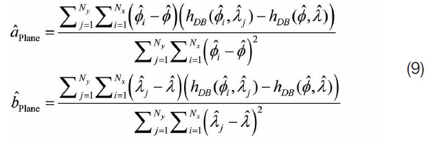
In comparison with the linear regression of Eq. (6), the longitude

is no longer fixed to the mean value in latitude slope estimation. The linearization error of planar regression is
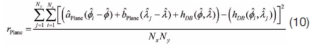
The planar regression method using a plane instead of two lines could reflect the correlation of two axes in terrain altitude. By doing so, estimated slopes could be estimated more accurately than using linear regression, and it could enhance filter stability.
3.2 Weighted Least Squares Method
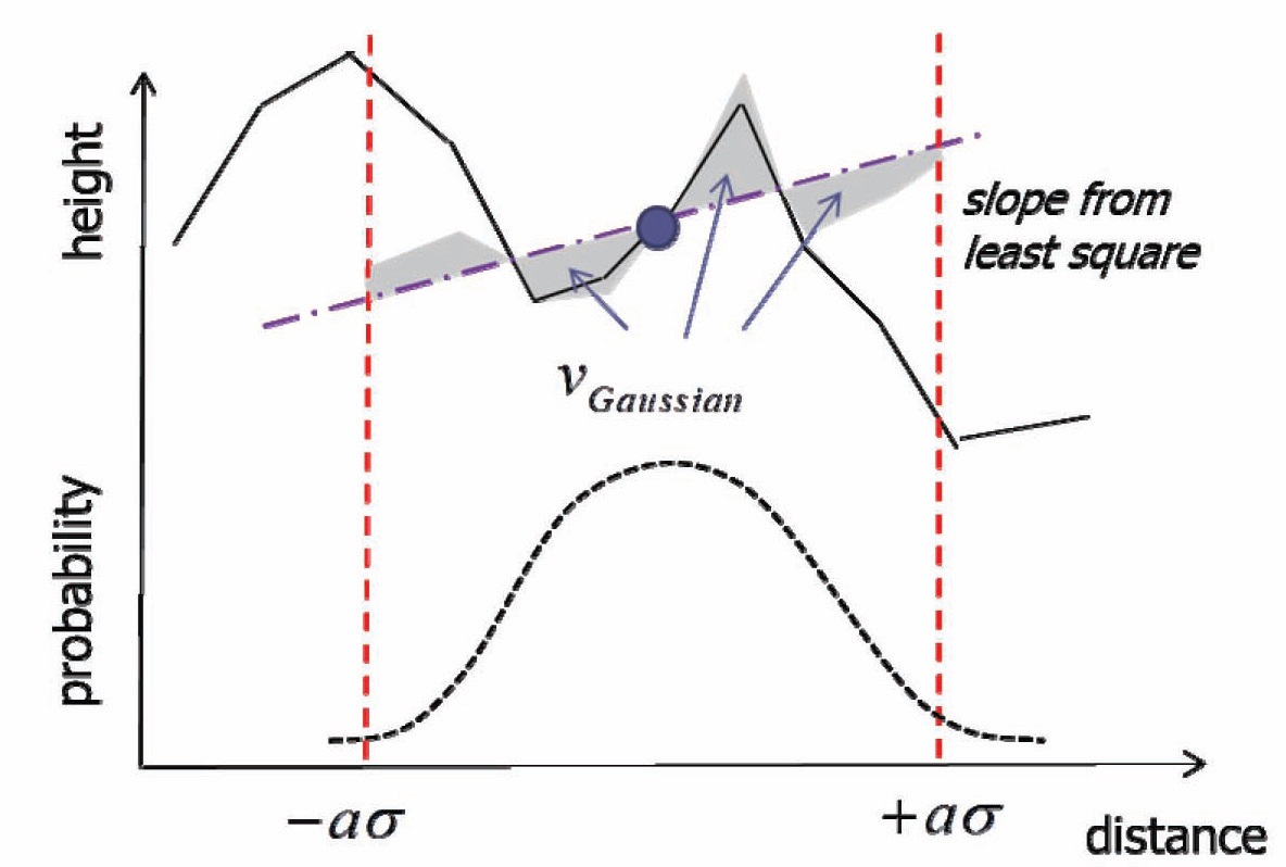
In a Kalman filter, the state is estimated based on a Gaussian probability density function (pdf). This characteristic could be applied in terrain slope estimation. In Eq. (8), the square of residual error is computed at each position in the linearization region. However, the probabilities of the estimated positions are different. To incorporate the difference, a Gaussian pdf can be utilized to generate a weight term at each position. By augmenting the weight, Eq. (8) can be modified to a weighted least squares problem, as
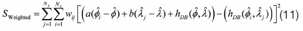
where,
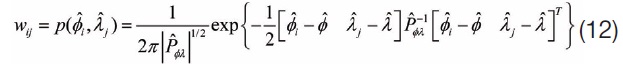

is a 2×2 matrix consisting of the estimated position
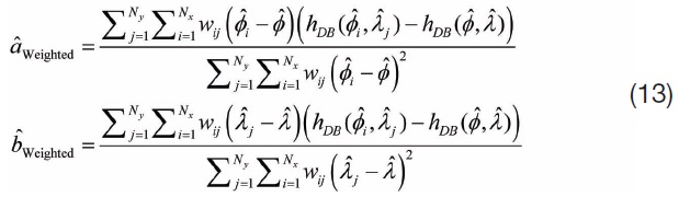
covariance. The corresponding optimal slopes, and variance of linearization errors, are given by
Figures 2 and 3 depict the two slope estimation methods, unweighted least squares (LS) and weighted least squares (WLS). The estimated slopes are different, in spite of the same terrain and position covariance. The weighted residual error is represented by the shaded area. We can see that the weights are even in LS, whereas larger weights are multiplied for adjacent regions in WLS. From a probabilistic view, the probability that the true position is in the near region is higher, than in the far region. So, commonly, the slope of WLS could be more accurate than that of LS, and the filter convergence speed could be faster. However, the true position might be distant, and in that case, the conservative LS solution could be more applicable in maintaining filter stability. In fact, the true position is unknown, so in the next section, Monte
Carlo simulation is conducted for various position errors, to compare the filter stability and convergence time between the two methods.
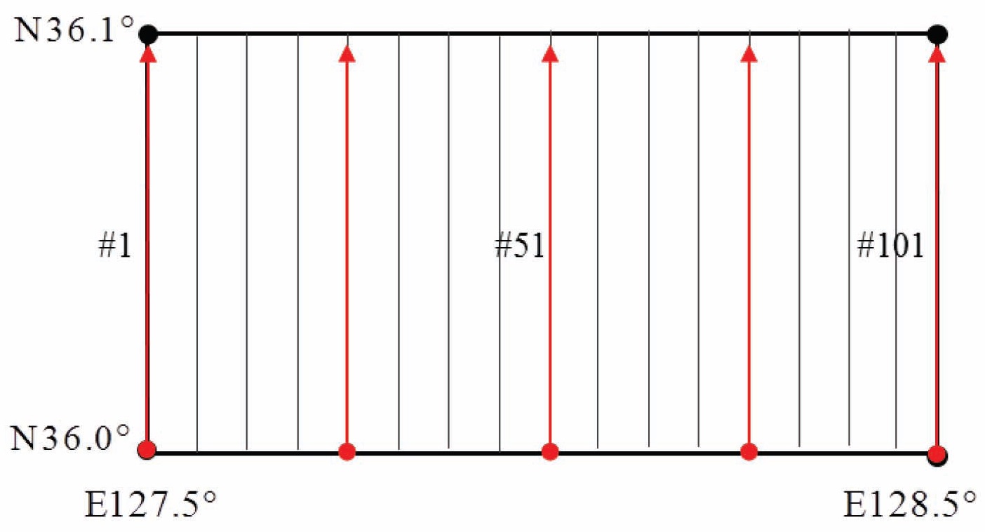
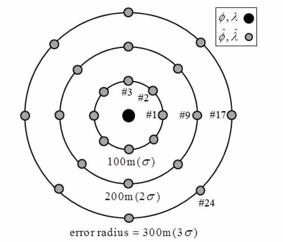
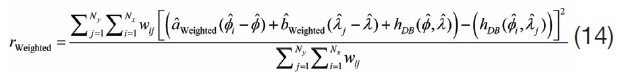
The two proposed methods, planar regressions with unweighted and weighted least squares, are applied in artificial missions. Monte Carlo simulation is performed by varying the initial position, and estimated error of the initial position. Figure 4 describes 101 mission trajectories, with various starting points. The other simulation conditions are summarized in Table 1. Initial position errors at each starting point are drawn in Fig. 5. Eight samples are positioned in each error radius, defined by multiplication of the estimated standard deviation of the position error
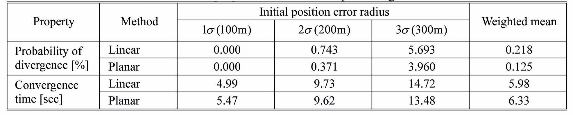
A performance comparison between the linear regression and planar regression is conducted. Table 3 represents the probability of filter divergence and convergence time according to the initial error radius in EKF, with the two methods. The convergence is defined as the position error in some boundary after a certain time, called the convergence time. In this simulation the grid distance of the map, 90m, is applied as the boundary. The last column in Table 3 denotes the weighted means of results at each initial error. A Gaussian pdf is applied as weights, and the values are 0.242 at 1
In Table 3, the probability of divergence increases as the position error grows, because the difference between the slopes at true and estimated positions becomes
[Table 1.] Simulation conditions
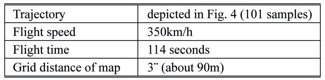
Simulation conditions
[Table 2.] Initial state errors
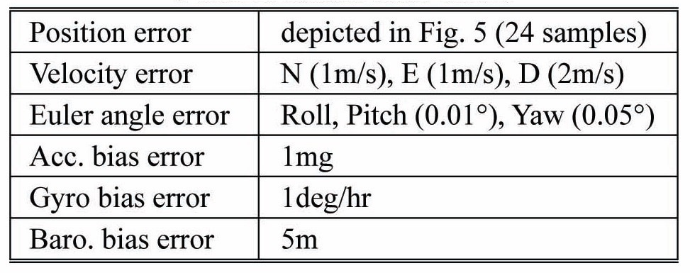
Initial state errors
[Table 3.] Filter properties of linear and planar regressions

Filter properties of linear and planar regressions
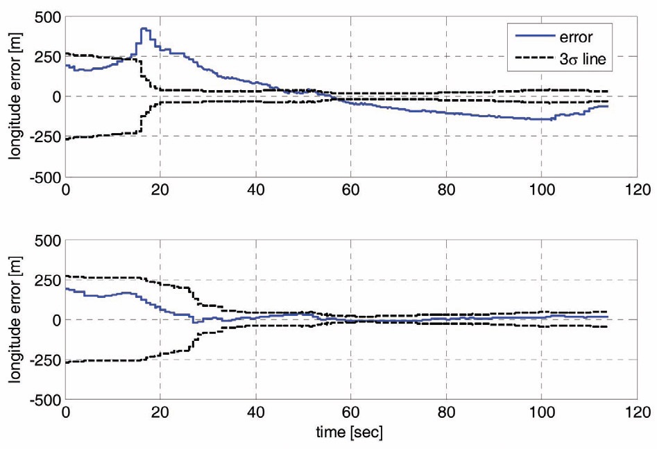
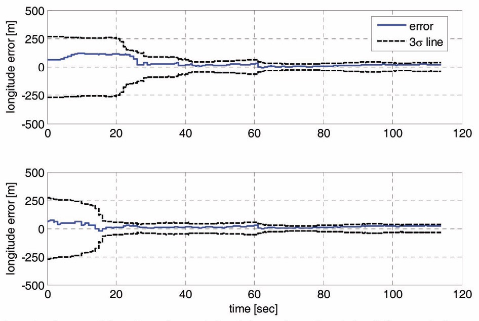
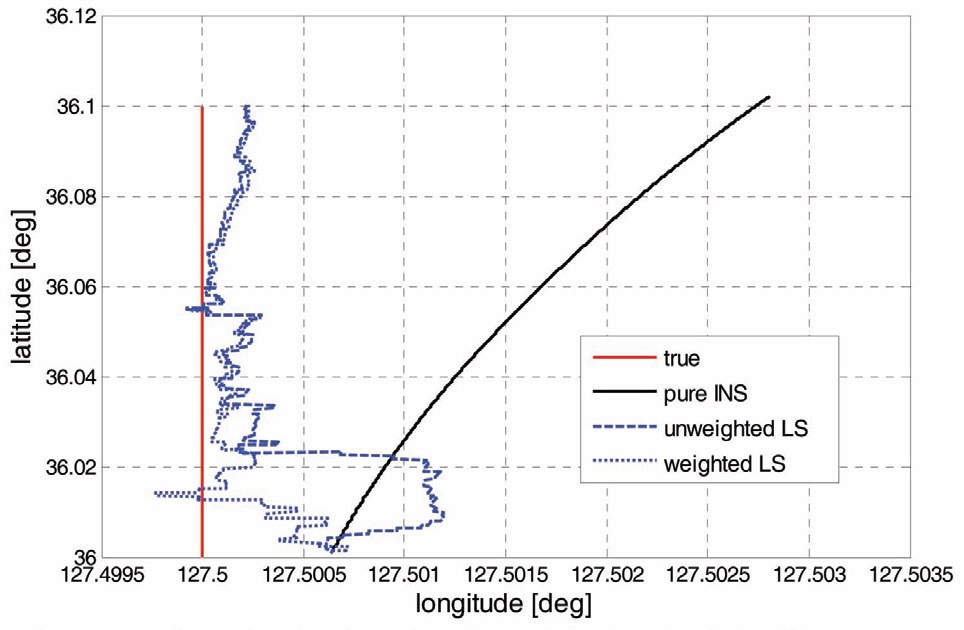
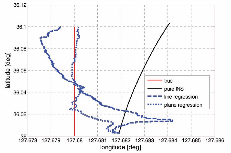
larger. Between the two slope estimation methods, the convergence times are similar, but the divergence probability is significantly reduced when the planar regression is employed. The simulation verifies that the slope could be estimated more accurately by using a plane, instead of two lines, and filter stability could be improved. Figures 6 and 7 describe the longitude error histories and planar trajectories at specific conditions, at 127.68° longitude and 300m initial error. In Fig. 6, the longitude error is well-bounded by the 3-sigma line with planar regression, but the filter is inconsistent and unstable in linear regression. The convergence characteristics can also be found in Fig. 7.
4.2 Weighted Least Squares Method
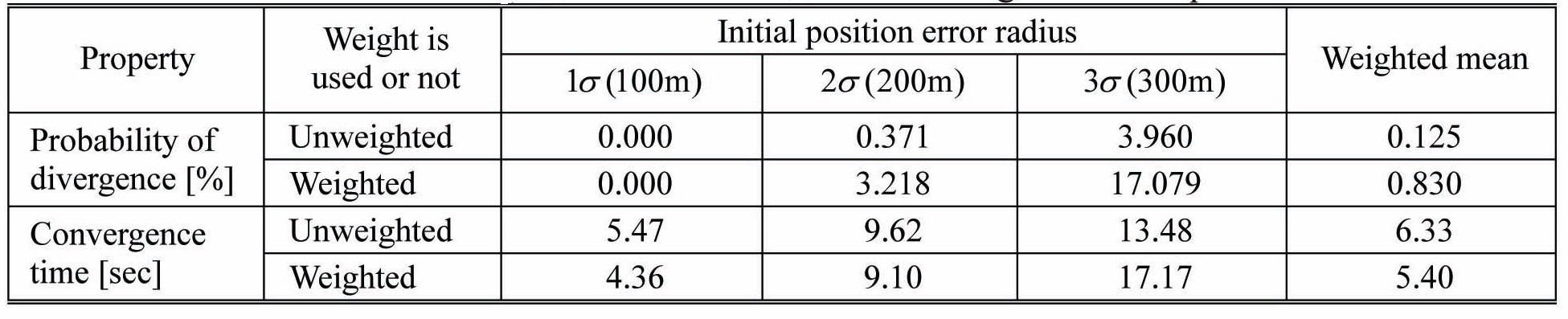
The filter properties of planar regressions with unweighted least squares (LS) and weighted least squares (WLS) are shown in Table 4. Simulation conditions and initial errors are summarized in Tables 1 and 2. In addition, the results of LS in Table 4 are identical with the planar regression results of Table 3. In Table 4, the convergence time is reduced about 20% in the smallest initial error 1
[Table 4.] Filter properties of unweighted and weighted least squares

Filter properties of unweighted and weighted least squares
speed faster. Figures 8 and 9 represent longitude errors and trajectories with 1
However in Table 4, as initial error increases, the difference of convergence speeds shrinks, and the divergence probability of WLS rises more rapidly than of LS. The less stable performance than LS in large initial error is because the WLS applies small weights for the far region. For the large error case, slope estimation with LS could be more effective in preserving filter stability. In summary, the superiority between LS and WLS depends on the initial error magnitudes. In the last column in Table 4, two filter properties are averaged over various initial errors. Overall, the probability of divergence is lower with LS, but the convergence speed is faster with WLS. One of the slope estimation methods could be implemented, after determining which of the filter properties is more significant, at each mission.
Terrain slope estimation methods based on least squares are developed. One is the planar regression, which improves upon the previous linear regression, and the other is the weighted planar regression, which adds Gaussian-shaped weights to the proposed planar regression. Two Monte Carlo simulations are conducted to compare the performances between the previous and two proposed methods, by considering the filter divergence probability and convergence speed. In the first simulation, the probability of divergence is reduced, when planar regression is employed instead of linear regression. In the second simulation, the performance difference between planar regressions with weighted and unweighted least squares changes, as the initial error radius varies. After taking the averages over various initial errors, it is shown that the convergence time is shorter with weighted least squares; but the probability of divergence is lower with unweighted least squares. By considering which of the filter properties is more important at missions, either of the proposed slope estimation methods could be implemented.