Since the recent slowdown in the smartphone market, studies for wearable devices are briskly being carried out to find new markets, such as virtual reality devices. In this paper, a head-mounted display (HMD) which provides expanded virtual images before human eyes by enlarging images of a small display was designed, and the tolerance analysis method for a focus-adjustable HMD based on afocal optical systems was studied. There are two types of HMDs: a see-through type that allows the user to view the surroundings, and a see-close type where the user can only view the display screen; the former is used in this study. While designing the system, we allowed a lens within the system to be shifted to adjust its focus from +1 to −4 D (diopters).
The yield of the designed systems was calculated by taking the worst-case scenario of a uniform distribution into account. Additionally, a longitudinal aberration was used rather than MTF for the tolerance analysis with respect to system performance. The sensitivity of the designed system was calculated by assigning a certain tolerance, and the focus lens shift was calculated to adjust the image surface variations resulting from the tolerance. The smaller the tolerance, the more expensive the unit price of the products. Very small tolerances may even be impossible to fabricate. Considering this, the appropriate tolerance was assigned; the maximum shift of the focus lens in which the image surface can be adjusted was obtained to find the changes in aberration and a good yield.
Since the recent dramatic growth slowdown in the mobile phone market, studies of wearable devices are actively being carried out to find a new market for wearable devices. Among the many types of wearable devices, the head mounted display (HMD) could be one of the most approachable products in the optical field [1]. According to Tractica, a foreign professional research center, virtual reality-related markets for HMD products are expected to grow explosively, to up to 21 trillion KRW by 2020 [2]. The HMD is a kind of viewfinder applied optical system where the optical part is detached from the camera to be worn on the face [3]. There are two types of HMDs [4]: a see-through type which allows the users to view the projected images, as well as to realize the augmented reality; and a see-close type where the user can only view the virtual reality on a display screen.
The HMD proposed in this paper must have the smallest size and weight possible to be worn on a face like glasses. Therefore, we used plastic materials for less weight and included the least number of lenses for smaller size. In Korea, people aged 65 or older reached 13.2% of the total population in 2015, and we are rapidly entering into an aging society [5]. For effective use by elderly people with presbyopia, whose crystalline lens has lost its elasticity and flexibility due to aging, a focus-adjustable product design was adopted in this paper. After considering the proper size of the product, the proposed system was designed to realize the same sensation as watching a 56" screen from a distance of 2 m, which corresponds to a field of view (FOV) of approximately 40°. In addition, the product must be focus-adjustable because each person has unique eyesight. Therefore, the system to be designed in this paper must have a lens that can be shifted to adjust its focus while the overall length of the product remains the same.
Measurement differences between designed parts and fabricated parts are called errors, and the error factors may be divided into symmetric and asymmetric ones. The symmetric error factors are the errors with respect to rotational symmetry about an optical axis, such as the number of Newton fringes, thickness, refractive index errors, etc., and the asymmetric error factors are the ones with no symmetry with respect to an optical axis, which are caused by lens tilt and apparatus fabrication errors, such as decentering, tilt, etc. [6]. Here, the error factors affecting the back focal length (BFL) include only symmetric error factors such as curvature of each side, thickness, and index. [7]. Only the rotational symmetric tolerance was calculated in this paper, and the focus-adjusting lens was shifted in order to adjust the image surface variations resulting from the symmetric error factors.
In order to evaluate mass production in terms of pricing, a tolerance analysis for afocal optical systems, such as HMDs, was performed to determine the fabricating errors of the acceptable parts, and the corresponding yield was calculated [8]. The design technique and tolerance analysis method for the afocal optical system proposed here may be applied to other fields, and this method can be widely used in camera viewfinders, not to mention HMDs, and afocal system products [9]. Besides HMDs, some afocal optical systems may also be applied to Head Up Displays (HUDs), which reflect the enlarged screen of a small image element onto a windshield [10]. Moreover, the basic design method of HMD optical systems can be used as is because the optical system used for the Fundus camera, which is not an afocal system but a retinoscope, is similar to an HMD optical system [11]. Therefore, this paper will specifically describe how to develop an HMD optical system, and related applications that are highly marketable, for tolerance analysis.
2.1. Definitions of Afocal Optical System and Aberration
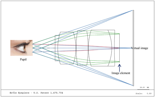
The rays from an object go through an eye-piece system, enter the human eye, and then focus on the retina, and here the eye works as a video receiver [12]. To see the object and focus the images on the retina, the rays must be parallel to the eyes. An optical system which allows the parallel light to be incident on the last surface of the optical system (the eye) is called an afocal optical system [13].
In Fig. 1, the eye is located where the stop is, and the image element is placed where the image surface is. A virtual image is seen as the image hits the retina after the image ray passes through the optical systems and reaches the stop, almost parallel to the eye. The larger the diameter of the stop, the wider the range of eye movement, which makes for easier viewing of the image; yet, this increases the design difficulty. In general, the diameter of the person’s pupil under an interior reading light is about 2 mm. However, considering the movement of the eye, we propose the stop size of the Type A design to be 8 mm and that of Type B to be 6 mm, as will be shown in Chapter 3.
In the afocal optical system, the lateral aberration is expressed in the angular difference between the chief ray and an arbitrary ray for aberration calculation at the stop surface, where the aberration is expressed in angular units [14]. Thus, the reciprocal of the distance between the stop surface and the convergence point of the chief and the arbitrary rays needs to be utilized. In general, the longitudinal aberration is expressed in diopters, the reciprocal of the meter unit, in the afocal system.
2.2. Calculating Lens Shift Using Longitudinal Sensitivity
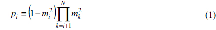
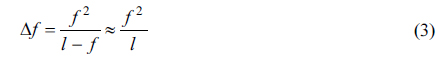
The Gaussian bracket is used to calculate the exact lens shift, but the longitudinal sensitivity may be used for an approximate calculation when the lens shift is minimal. Because the lens shifts very little while correcting the variation of the image surface in this system, we used the longitudinal sensitivity to calculate the approximate lens shift. Eq. (1) is used for calculating the longitudinal sensitivity, where

2.3. Calculating Tolerance and Sensitivity of Design Variables
In a product fabrication with design data determined by the optical design, the actual production of the product is not in general the same as originally designed due to the limitations of the fabricating and assembly precision of the parts. If an error occurs during the fabricating stage of the product, the resolution, such as the modulation transfer function (MTF), usually becomes lower than the designed value. However, a lower resolution than designed does not necessarily mean it is defective. Despite the somewhat lower resolution performance, the product can be regarded to be of fair quality if it meets the initial target performance. The optical system is designed to have a higher performance than the initial target during the design stage in order to compensate for the performance degradation. The maximum limit of acceptable errors to satisfy the target optical performance is called the tolerance.
Only the symmetric tolerance was calculated in this paper and the symmetric tolerance factors include the curvature, thickness, and refractive index, which are the major design variables of the optical system. Because the aberration changes by the tolerance are minimal in this paper, having very little effect on the yield, we only considered the yield with respect to the BFL. In addition, the performance changes of the systems when a certain tolerance is applied to the design variables are called the sensitivity, and the yield of the product can be calculated using the system sensitivity with respect to each tolerance.
The system performance can be determined by the sensitivity analysis with respect to the tolerance. Here, we used the longitudinal aberration rather than the MTF to obtain the system performance because it is much faster to calculate the aberration than the MTF, and the performance changes from the errors at each surface can be linearly summed.
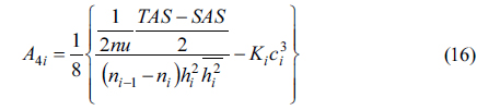
Eq. (4) is an expression for the BFL in terms of the curvature, thickness, and refractive index. Eq. (4) can also be expanded using a Taylor expansion of the design variables. Here, the Taylor expansion must be expanded using the given initial design values, where,
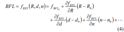
The number of terms in Eq. (4) will increase depending on the lenses in the optical systems. In order to find out the performance changes, however, the variation in the image surface (
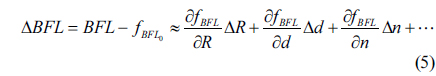
There are spherical aberrations, which degrade the on-axis resolution, and astigmatism, which compromises the off-axis resolution. Besides, if the optical system, like HMD, has a large distortion, the screen will look as if it rotates depend on the variation of the pupil position. This is called the swing phenomenon, which causes dizziness when wearing an HMD optical system. This phenomenon is similar to the keystone that occurs in the projection system [17]. Therefore, distortion should also be included as one of the evaluation factors in an HMD optical system even though it does not lower the resolution. Along with the BFL, spherical aberration, astigmatism, and distortion should be added to the performance evaluation factors. In Eq. (5), spherical aberration, astigmatism, and distortion should be considered rather than the BFL for the same calculation, and the sensitivity for each design variable must be calculated. However, due to the nature of the afocal optical system, the eye focuses on each image surface, and almost no performance degradation from the image surface curvature is detected, so it can be omitted.
2.4. Calculating Yield of the Optical System
Even if each lens and device part is fabricated or assembled within the tolerance in general, assembling those parts without additional adjustments would cause performance degradation and lead to a low yield. As a workaround, and to increase the yield, the value of an arbitrary design variable is adjusted to correct the image surface shift and aberration changes. Among the many design variables of the optical systems, the curvature and refractive index cannot be used as adjustment variables in this paper because they are fixed in the product fabrication stage. The HMD optical system to be designed in this paper has a movable lens for focus adjustment. By using this, the image surface shift and aberration changes due to the tolerance will be adjusted. Here, the space before and after the movable lens must satisfy the values for the focus adjustment as well as for the performance adjustment. If the space is not enough, the tolerance range must be reduced. If the tolerance range cannot be reduced due to the fabrication technique limitations or cost, the optical system must be redesigned. The greater the tolerance range, the easier it is for parts fabrication and assembly, which enables the lower unit price; however, the optical system performance will be compromised. Therefore, the appropriate tolerance level should be assigned by considering the cost of production as well as fabrication and assembly techniques.
The product error, on the other hand, would have a statistical distribution for the quantity and quality management of the products, where Δ
Even if the design variables, such as the fabrication and assembly errors of the parts, follow the uniform distribution, the performance distribution for the changes of the overall design variables will follow the normal distribution by the central limit theorem [22]. The top quality management level in the mass production stage would be achieved when the standard deviation of the statistics following such a normal distribution becomes 1/6 that of the range of acceptable performance; that is, when the range of acceptable performance is six times the standard deviation of the performance distribution [23]. Considering the unknown causes of fabrication errors at this point, the average of the performance distribution may be slightly different from the design values. In general, an average shift resulting from the unknown causes of fabrication errors of as much as 1.5 times the standard deviation (σ) is acceptable in the quality management [24]. Taking into account the average shift in reality, the highest level of quality management would be achieved when the acceptable performance range become 4.5 times the standard deviation of the performance distribution [24]. This corresponds to 6.7 defective parts per million (DPPM); that is, a theoretical minimum defective percentage [24]. If enough lens shift distance can be obtained to adjust the Δ
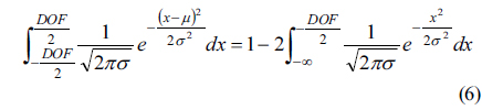
Two types of optical systems were designed in this paper: Type A, which is relatively large, and Type B, which is relatively small, as will be shown in Chapter 3. The yields of Type A and Type B can be calculated with Eq. (6), where
The optical system in this paper was designed to compensate the
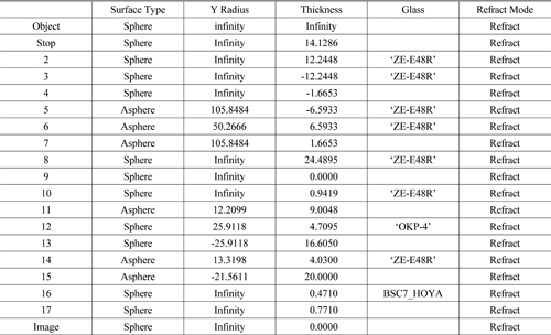
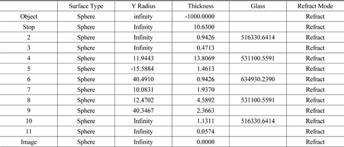
Based on the data for the initial optical system in Tables 1 and 2, the Type A optical system was determined [26]. The Type A is an optical system with a diagonal HFOV (Half Field of View) 20 degrees and its specifications include an entrance pupil diameter of 8 mm, and an HD (1280 × 720) level of pixels. The distance between the human eye and the first lens from the eye is called the eye relief [27]. The eye relief was set to 15 mm to allow for glasses wearers to use it as well. For the optical layout in Fig. 2, an image from an image surface is focused on the inner part of a beam splitter by a relay system, then the rays are collimated at the stop after passing through the optical parts with the reflector.
[TABLE 1.] Initial data for Type A
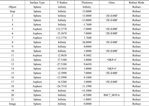
Initial data for Type A
[TABLE 2.] Initial aspheric data for Type A
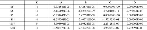
Initial aspheric data for Type A
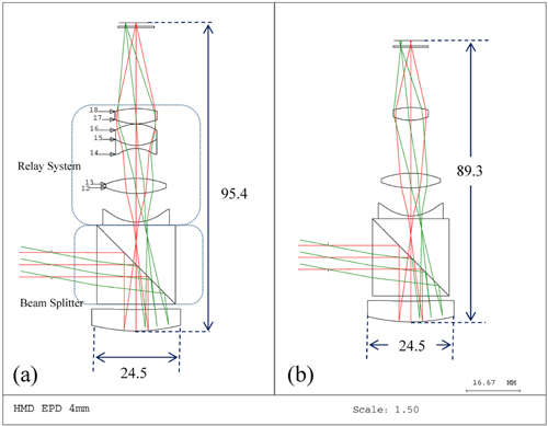
Figure 3(a) is the layout of the optical system with an adjusted ratio of image size: the EFL to meet the system specifications before designing the Type A. Moreover, in order to design the smallest possible optical system, the refracting power of the cemented and above convex lenses (14th to 18th surfaces) was set to be identical to be that of the cemented lens and the above single convex lens (17th to 18th surfaces); they were replaced with a single lens. Figure 3(b) is the optical layout of the system where the refracting power of 14th to 18th surfaces is replaced with a single convex lens (17th to 18th surfaces).
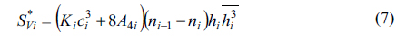
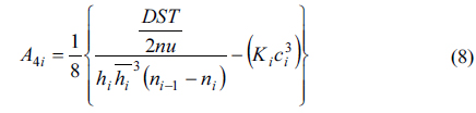
An aspherical lens was used instead of a spherical lens to correct the distortion, and the 4th order aspherical coefficient was calculated to make the Seidel aberration for the distortion zero. Distortion (
In Eq. (7), Seidel aberration coefficient
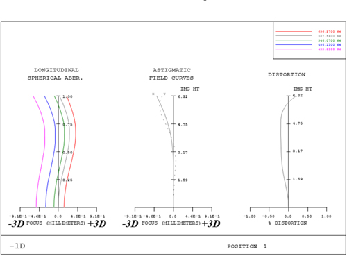
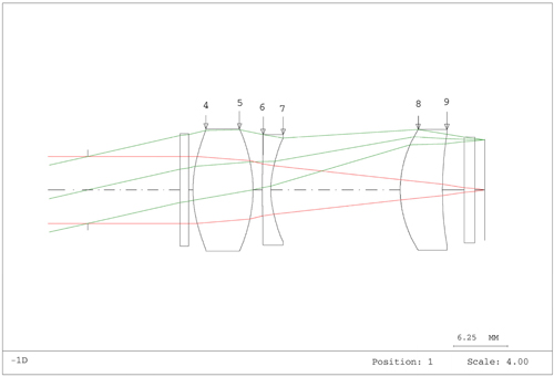
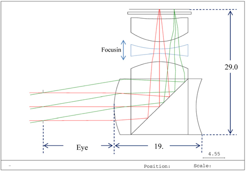
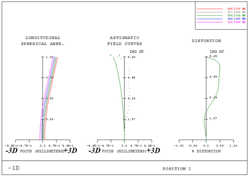
The calculated 4th order aspherical coefficient of the 12th surface is −0.147850, and the 3rd order distortion after applying this value is zero. By applying the lens data in Table 3 and the 4th order aspherical coefficient of the 12th surface, the initial design data of the Type A were obtained. The design data in Tables 4 and 5 were also obtained through optimization, and the optical layout of the final Type A is shown in Fig. 4. The final system was designed to be smaller than the initial system in Fig. 2 (overall length of 101.27 mm, beam splitter length of 26 mm). Type A was designed within −4 D to +1 D to allow focus adjustment, and Fig. 5 shows the layout of the longitudinal aberration of Type A in the case of −1 D.
[TABLE 3.] Data for system with one lens replacement
Data for system with one lens replacement
[TABLE 4.] Data for final Type A
Data for final Type A
[TABLE 5.] Aspheric data for final Type A
Aspheric data for final Type A
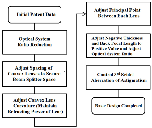
The flow chart in Fig. 6 describes the design process for Type B. The Type B system is designed based on an existing viewfinder patent (JP2012-093478 EX1). The optical layout as shown in Fig. 7 can be obtained when the patent information is applied. The specifications of the Type B are the same as that of the Type A, i.e., EFL of 17.5 mm, eye relief of 15 mm, and HD. However, because of decreased freedom in the design for using fewer optical surfaces, the Type B was designed to have a smaller diameter of the entrance pupil (EP) of 6 mm, compared to the Type A. First, the image size and EFL ratio were adjusted to meet the target specifications of the system. Here, it is important to adjust the ratio of the surface next to the stop to avoid a possible decrease in eye relief. Because the initial data for Type B mainly consists of the radius of curvature, thickness, and refractive index, the surface type of every surface is changed to a spherical one.
The thickness of the biconvex lens (4th-5th surfaces) was increased to 10 mm discretely to ensure the space for a beam splitter. It will change the EFL of the biconvex lens; to keep the EFL the same as before the thickness change, the curvature of the front or back surface of the biconvex lens must be changed. To do so, the EFL equation for a thick lens is used to find the accurate curvature of the front or back surface of the biconvex lens. From the two choices of curvature between the front (4th) and back (5th) surfaces of the biconvex lens, the curvature of the surface with the smaller ray refraction angle should be chosen to ensure little change in the performance. Since the front (4th) surface of the biconvex lens has a relatively smaller ray refraction angle, the curvature of the front surface can be changed to realize the existing EFL before the thickness of the beam splitter is increased.
Eq. (9) is an equation of the EFL for thick lenses, and this can be used to obtain Eq. (10). In Eqs. (9) and (10),
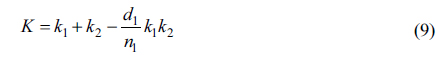
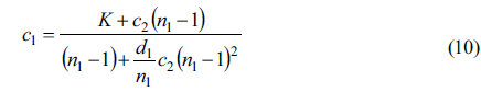
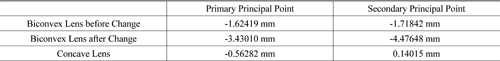
Using Eq. (10), the radius of curvature of the front surface of the biconvex lens was found to be 8.651 mm so that the EFL would have the same value as before changing the thickness of the beam splitter. However, because the curvature and thickness of the biconvex lens were changed, the distance of principal points between the biconvex lens and the concave lens would also be different from that of the initial system. To maintain the characteristics of the initial system, the distance between the two lenses must be adjusted to correct the position of each lens with the interval of the principal points of the initial system. Table 6 shows the principal points of the biconvex lens before and after the change, as well as the principal points of the concave lens.
[TABLE 6.] Principal points of the biconvex lens and concave lens
Principal points of the biconvex lens and concave lens
The distance between the secondary principal point of the biconvex lens before changing its properties and the primary principal point of the concave lens is 2.99768 mm; and the distance between the secondary principal point of the biconvex lens after changing its properties and the primary principal point of the concave lens is 5.75573 mm. Because of the increased distance of 2.75805 mm between the principal points, the thickness at the 5th surface, the distance between the biconvex lens and concave lens, was reduced by as much as 2.75805 mm to make it the same as the distance between the principal points of the initial system.
Although the overall EFL of the current system was set at the initial design target of 17.5 mm, the thickness of the 5th surface between the biconvex and concave lenses turned out to be a negative value of −2.04162 mm. In this case, physical fabrication of the product would be impossible. Therefore, the thickness should be adjusted to an arbitrary positive number. To do so, the distance between the biconvex lens and the concave lens needs to be adjusted to an arbitrary value and the Gaussian bracket is used to keep the overall EFL unchanged. Then, the thickness between the concave lens and the meniscus lens (8th-9th surfaces) can be found.
Here, in Eq. (11),
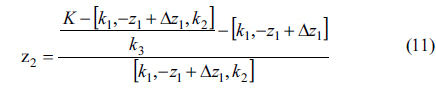
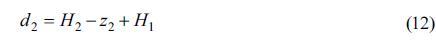
Here, 3.1 mm is added to the thickness of the 5th surface, the gap between the biconvex lens and the concave lens, to ensure an approximately 1 mm space for focus adjustment with the concave lens. In Eq. (12),
[TABLE 7.] Data for adjusted Type B
Data for adjusted Type B
In order to have a system with minimized aberration, the aspheric 4th order coefficient was used to adjust the 3rd order aberration. The curvature of the field is not important due to the characteristics of the afocal system, thus other aberrations except the curvature of the field were adjusted. However, if the spherical aberration, coma aberration, astigmatism, and distortion are all adjusted, it would not be easy to fabricate the shape of the system; thus, only the 3rd order aberrations for the three types of aberration except the spherical aberration, which is relatively small, were adjusted. The aberrations to be adjusted in the present optical system include the tangential coma (TCO) of −0.533186 mm, tangential astigmatism (TAS) of −1.301066 mm, sagittal astigmatism (SAS) of −0.528742 mm, and DST of −1.110859 mm. The TCO and DST need to be adjusted to zero, and the SAS and TAS to have the same value.
In Eq. (13),
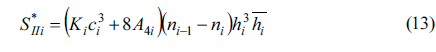
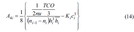
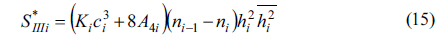
To adjust the Seidel aberration using the aspherical coefficient, just the
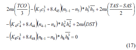
As shown in Fig. 8, the aspherical coefficients where the TCO and DST are zero and the difference between TAS and SAS is zero are
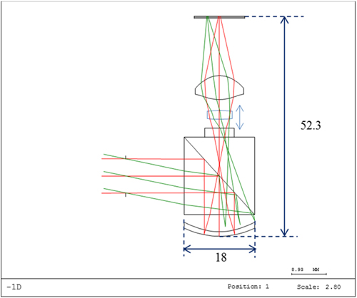
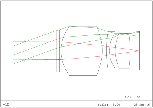
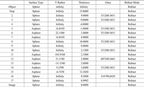
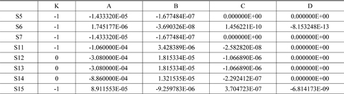
The lens data in Table 7 and the 4th order asphericities at the 4th, 5th, and 8th surfaces were used for the initial design data of the Type B system. Afterwards, these data were optimized to design the Type B. Table 8, Table 9, and Fig. 10 show the design data and the layout of the final Type B system. The Type B is also a focus-adjustable design in the range of −4 D to +1 D, and Fig. 11 is the longitudinal aberration layout of the Type B in the case of −1 D. Table 10 shows the comparison between the Type A and Type B.
[TABLE 8.] Data for final Type B
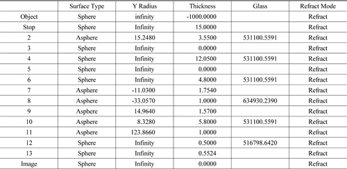
Data for final Type B
[TABLE 9.] Aspheric data for final Type B
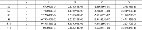
Aspheric data for final Type B
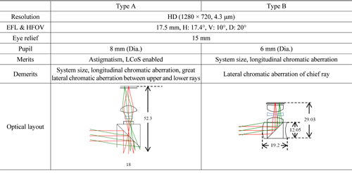
Type A vs. Type B
3.3. Calculating Lens Shift Using Longitudinal Sensitivity
Using Eqs. (1)-(3), the longitudinal sensitivity, image surface shift at 1 D, and lens shift of the Type A and Type B can be calculated. The Type A and Type B systems in this paper were designed to be focus-adjustable within −4 D to +1 D, where the image surfaces of each system were shifted by as much as 0.3142 mm and 0.35949 mm, respectively, as the image surface (image sensor in this case) changed by up to 1 D. Table 11 shows the image surface shift and lens shift due to the change of 1 D, which is calculated using the longitudinal sensitivity and DOF.
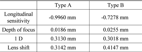
Longitudinal sensitivities, DOFs, image surface changes, and lens shifts for Types A and B
IV. CALCULATING TOLERANCE AND YIELD
4.1. Calculating Tolerance and Sensitivity of Design Variables
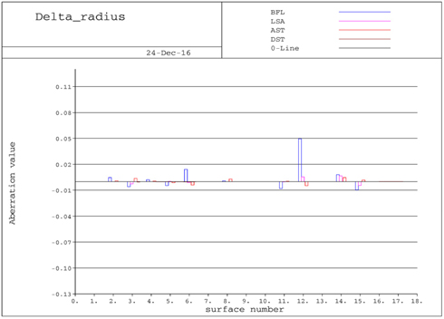
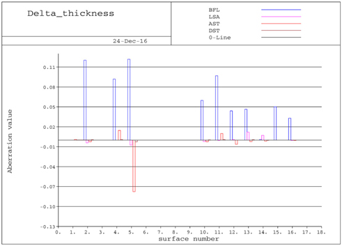
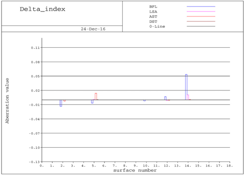
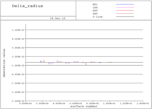
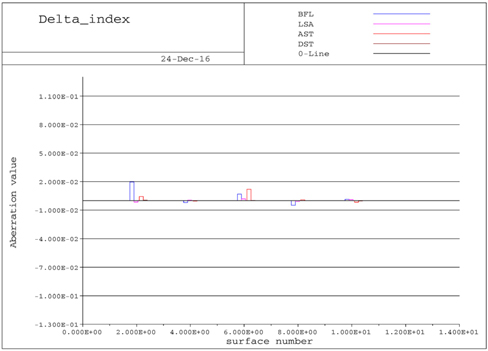
Figures 12 to 17 show the aberration changes when a certain tolerance is assigned to the designed optical systems. When the tolerances of the five-fringe Newton Ring for the radius of curvature, 0.05 mm for the thickness, and 0.001 for the refractive index were assigned, the changes of each aberration can be expressed in terms of the sensitivity for each tolerance. Here, the material of the cover glass is BSC7 by the Hoya Corporation, which allows a tolerance of 0.0003. Because the off-axis does not carry more weight than the on-axis in general, the sensitivity data was calculated at the area where its FOV is 0.8 times that of the object side. Table 12 lists the standard deviations of the Type A and Type B, which can be used to calculate the yield.
[TABLE 12.] Standard deviations of Type A and Type B

Standard deviations of Type A and Type B
Since the variations of longitudinal spherical aberration and astigmatism are all less than 1 D and maximum changes in the distortion (−0.270%, +0.084%) are very little for both Type A and Type B, they have little effect on the yield. However, the standard deviations of the image surface shift were greater than the depth of focus (Type A: 0.0186 mm and Type B: 0.0255 mm) affecting the performance changes, which might cause defective products. Therefore, only the image surface shift was considered to get the yield. Eq. (6) was used for the yield of Type A and Type B, and it can be calculated using the Norm.dist function in Excel. This function returns the normal distribution for the given average and specific standard deviation. As a result, Type A and Type B for the current image surface shift had yields of 5.05% and 17.36%, respectively. To increase the yield, the system was designed to adjust its focus-adjustable lens to correct the image surface shift in this paper, and Eq. (2) was used to obtain the lens shift when the image surface was changed by as much as 4.5
[TABLE 13.] Lens shifts of Type A and Type B
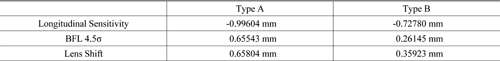
Lens shifts of Type A and Type B
A see-through type HMD optical system was designed to realize the augmented reality. Affordable plastic was used to lighten the system, and Type A system followed by Type B was designed in a smaller and different shape. In addition, a piece of lens was configured to be shifted from −4 D to +1 D for focus adjustment in order to compensate the individual eyesight.
Although fabrication errors are unavoidable during mass production, the product can be regarded to be of fair quality as long as the target performance is satisfied. The system yield was calculated after analyzing its sensitivity in relation to the tolerance, which is the maximum margin of error satisfying the system performance. Only the symmetric tolerance was dealt with in this paper, and a Newton ring of five fringes, thickness of 0.05 mm, and refractive index of 0.001 were assigned as the tolerances to analyze the sensitivity for each case. The system performance could be checked via the sensitivity analysis in relation to the tolerance, and a longitudinal aberration was used instead of the MTF. This was because the aberration can be calculated much faster than with the MTF, and the performance changes for the error at each surface can be linearly summed. The sensitivity analysis was performed on the longitudinal aberration and the variation of the image surface for the on-axis performance, and on the astigmatism and distortion for the off-axis performance. The yield was calculated only for the image surface shift with greater variation because the longitudinal spherical aberration, astigmatism, and distortion of Types A and B are relatively small. Here, a focus-adjustable lens was used to adjust the image surface shift for a greater yield. Because the shift in axis for the standard deviation was assumed to be 1.5

![Example of an afocal system [13].](http://oak.go.kr/repository/journal/21630/KGHHD@_2017_v1n5_474_f001.jpg)