Stereoscopic (S3D) displays present different images to the two eyes. Temporal multiplexing and spatial multiplexing are two common techniques for accomplishing this. We compared the effective resolution provided by these two techniques. In a psychophysical experiment, we measured resolution at various viewing distances on a display employing temporal multiplexing, and on another display employing spatial multiplexing. In another experiment, we simulated the two multiplexing techniques on one display and again measured resolution. The results show that temporal multiplexing provides greater effective resolution than spatial multiplexing at short and medium viewing distances, and that the two techniques provide similar resolution at long viewing distance. Importantly, we observed a significant difference in resolution at the viewing distance that is generally recommended for high-definition television.
Resolution is an extremely important component of perceived image quality. Viewing distance is, in turn, important for determining resolution. For example, ITU-R Recommendation BT.709 states that “a high-definition system is a system designed to allow viewing at about three times the picture height, such that the system is virtually, or nearly, transparent to the quality of portrayal that would have been perceived in the original scene or performance by a discerning viewer with normal visual acuity” [1]. At a viewing distance of three times screen height (3 H), the pixel density of the high-definition (HD) format is 56.5 pixels/deg. That density corresponds to a pixel size of slightly more than 1 arcmin, which is considered by practitioners to be equivalent to normal (20/20) visual acuity for a healthy eye; specifically, someone with 20/20 acuity can just read letters with a stroke width of 1 arcmin. To display such letters on a digital device, each pixel should be no larger than 1 arcmin. The reasoning, therefore, is that HD format can properly display the smallest letters that people with normal acuity can read, at the recommended viewing distance.
Stereoscopic (S3D) displays have to show the images for both eyes in one stereo frame. Most S3D displays achieve this by multiplexing the two images either temporally or spatially. Temporal multiplexing alternates left- and right-eye images in time, while spatial multiplexing presents the left-eye image on odd pixel rows and the right-eye image on even rows. With temporal multiplexing, all of the image data are shown to the left eye and none to the right eye at one time, and then all of the image data are shown to the right eye and none to the left at another time. With spatial multiplexing, half of the displayed pixels are shown to the left eye and half to the right eye in a given frame. Because only half of the pixels are displayed, numerous investigators and practitioners have suggested that the effective resolution of such displays is reduced relative to temporally multiplexed displays. Others, in contrast, have argued that effective resolution in such displays is not reduced, because the brain fuses the two monocular images into a full-resolution binocular image [2, 3]. To find out which of these two accounts is more valid, we conducted a psychophysical investigation of how the multiplexing technique affects the effective resolution of the display.
There are two temporal-multiplexing methods [4]. In simultaneous-capture, alternating-presentation, left- and right-eye image data are captured simultaneously and presented alternately to the two eyes. In alternating-capture, alternating-presentation, left- and right-eye image data are captured and presented alternately to the two eyes. The two techniques only differ when the stimulus changes over time. In this paper we focus on stationary stimuli, so the distinction is not important.
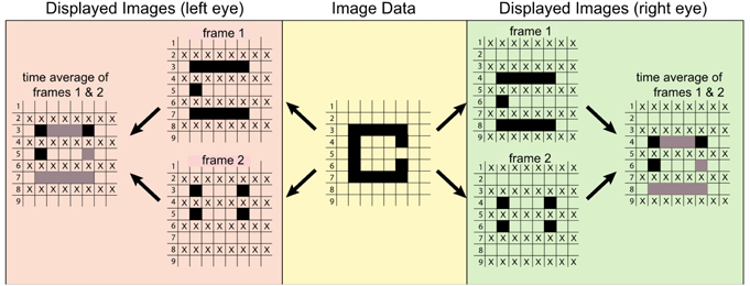
There are three spatial-multiplexing methods [5, 6]. From top to bottom in Fig. 1, they are same-line allocation, alternate-line allocation, and both-line allocation. In each row, the left eye’s image data are shown on the left and the right eye’s on the right. The displayed stereo image is in the center. Line 1 in the displayed image is visible to the left eye, and is either line 1 or line 2 from the left eye’s image data. Line 2 in the displayed image is visible to the right eye, and is either line 1 or line 2 from the right eye’s image data.
In same-line allocation, the same rows in the image data are shown to both eyes. Specifically, the odd rows displayed to the left eye contain data from the odd rows in the left eye’s image data, and the even rows displayed to the right eye contain the data from the odd rows in the right eye’s image data. The even rows of the image data are not displayed at all.
Alternate-line allocation recruits the rows in alternating fashion from both eyes’ image data. The odd rows in the left eye’s image data are displayed as odd rows to the left eye, and the even rows in the right eye’s image data are displayed as even rows to the right eye. The even rows in the left-eye image data and the odd rows in the right-eye image data are not displayed.
Both-line allocation presents image data from all rows. Pairs of rows in the left-eye image data are combined to be displayed in odd rows on the display, and row pairs in the right-eye image data are combined to be displayed in even rows. In one common implementation of this method, the data are allocated differently in two successive frames. In the first frame, odd rows in the left-eye data are presented to the left eye on odd display rows, and in the second frame even rows in the left-eye data are presented to the left eye on the same odd display rows. The same occurs for the right-eye data and display, but odd image data are first presented to even display rows. The alternating presentation of the pairs of image data rows is meant to happen quickly enough for the data to be temporally averaged by the visual system.
Kim and Banks [7] measured the effective resolution of temporal and spatial multiplexing techniques, and showed that it was higher with temporal multiplexing at viewing distances of 1.5 and 3 times screen height (respectively, 1.5 H and 3 H). Yun, Kwak, and Yang [8] compared grating visibility with both multiplexing techniques at a distance of 3 H, and found that higher spatial frequencies were visible with temporal multiplexing. However, these studies have two limitations. (1) They tested only one spatial-multiplexing method. Park, Kim, and Choi [9] tested same-line and alternate-line allocation, and found that perceived image quality was the same with the two allocation methods. They did not measure effective resolution. (2) They did not test at the currently recommended viewing distance of 3.2 H, where one pixel subtends exactly 1 arcmin at the viewer’s eye [10]. They also did not test at the viewing distance that is recommended by prominent TV manufacturers; for example, LG recommends a distance of two times the screen diagonal, which corresponds to 4.1 H.
In the current work, we addressed both of these limitations by testing different allocation methods for spatial multiplexing, and by testing at distances of 3.2 and 4.1 H.
II. EXPERIMENT 1: TV COMPARISON
We measured the effective resolutions of two commercial televisions, one using temporal multiplexing and the other using spatial multiplexing. The televisions were set to their default modes, so they differed somewhat in brightness, contrast, and crosstalk.
The temporal-multiplexing TV was a Samsung LED TV 8000 and the spatial-multiplexing TV was an LG 55LW6500. Both TVs were 55” on the diagonal with 1920×1080 resolution in 2D mode. Both were tested in their default stereo mode. We used the stereo glasses that came with the products. The luminance of the Samsung TV was 133 cd/m2 without stereo glasses, and 37 cd/m2 through the glasses. The luminance of the LG TV was 200 cd/m2 without the glasses, and 87 cd/m2 through them.
We provided 1920×1080 resolution images for the left and right eye views by enabling NVIDIA 3D Vision on our gpu (GTX 580). Both TVs recognized the protocol and presented the scene without any scaling or clipping. Of course, spatially multiplexing TV cannot provide lossless display of all of the provided pixels. However, that processing happened on the TV side, not on the control pc.
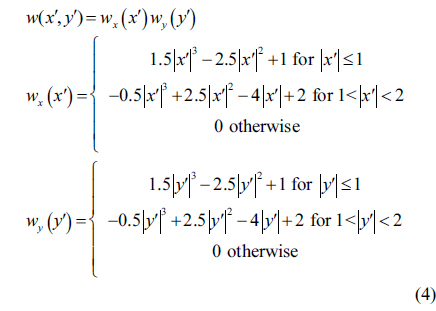
We used a letter acuity test to measure effective resolution. The stimuli were black capital letters from the English alphabet, presented on a white background (Fig. 2). They were created using the design of the letters in a standard clinical eye chart [11]. Letter height was five times greater than letter stroke width, letter width was four times stroke width, and the spacing between letters was twice the letter width. We pre-rendered high-resolution images (400×500) for the 26 letters of the alphabet. During the experiment, the pre-rendered images were resized as desired. We applied cubic interpolation for antialiasing, as described in the
We tested the two multiplexing methods at four viewing distances, yielding eight conditions. The spatial-multiplexing TV used both-line allocation. Each display row on this TV temporally alternated information from odd and even image rows, for a given two-frame sequence. This is equivalent to spatially averaging the two image rows, because the duration of each frame is only 1/120 s, short enough to be fused temporally by the visual system. Figure 3 illustrates this.
We conducted the experiment at four viewing distances: 1.59, 3.18, 4.08, and 6.37 H, which corresponded to 1.09, 2.18, 2.79, and 4.36 m, respectively. Table 1 shows the letter sizes presented at each of the viewing distances. The angular sizes of the letters were roughly the same at all distances, except for the shortest distance, where 3 arcmin was too small to be adequately presented using 2-arcmin pixels.
[Table 1.] Letter sizes presented at the four viewing distances
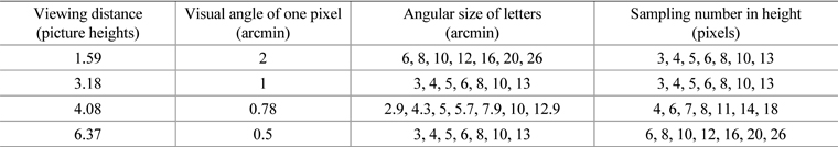
Letter sizes presented at the four viewing distances
We divided the experiment into roughly 15-minute sessions for different viewing distances and multiplexing methods. The order of sessions was randomized across subjects. After each session, subjects were free to take a break. The whole experiment took about two hours. A total of 3,018 identification responses were obtained from each subject.
On each trial, three letters were presented for 600 ms and then extinguished. This duration is sufficiently long for visual acuity to be maximized [12]. After the stimulus was extinguished, a uniform white stimulus appeared, and the computer awaited the subject’s responses before proceeding to the next trial. The subject identified the letters he or she thought were presented by making three keyboard responses, indicating the letters that appeared from left to right on the screen. The procedure was forced choice, meaning that the subject had to make three responses, whether he or she was certain or not. No feedback as to the correctness of the responses was provided. To make sure that the intended keys were pressed, larger versions of the letters associated with each response were written to the screen; the subject could retype a response if the intended key had not been pressed. When the subject was satisfied with the responses, he or she pressed the space bar to proceed to the next trial.
Six young adult subjects, 24 to 36 years old, participated. All had normal or corrected-to-normal visual acuity and stereoacuity. If they would normally wear corrective lenses, they wore them behind the 3D glasses during the experiment. All but one were naïve to the purposes of the experiment.
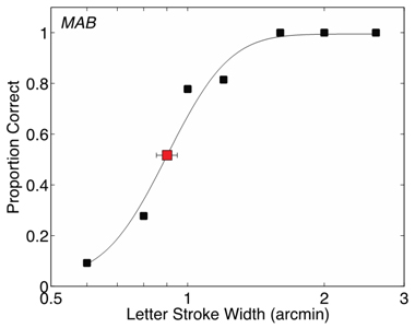
We plotted the proportion of correct identification responses as a function of letter size, for each condition. Figure 4 shows data from one subject at one viewing distance. The solid line represents the cumulative Gaussian function that best fit the data:

where
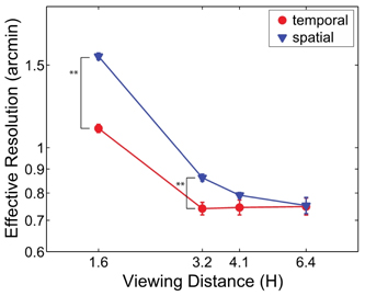
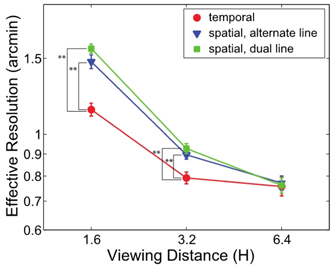
The data were very similar across subjects, so we averaged them. Figure 5 presents the effective resolution estimates for both multiplexing techniques and all four viewing distances, averaged across subjects. At 1.6 H and 3.2 H, perceived resolution was significantly better for temporal than for spatial multiplexing (
III. EXPERIMENT 2: CRT SIMULATION
The images presented on the two televisions in Experiment 1 differed somewhat in brightness, contrast, and crosstalk. We wanted to make sure that those differences did not cause the observed differences in effective resolution. Therefore we conducted a second experiment in which we simulated the two multiplexing techniques on the same display.
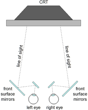
The stimuli were presented on one CRT display using a mirror stereoscope (Fig. 6). By using one display, we could make the luminance, contrast, and crosstalk (in this case there was no crosstalk) identical across conditions. The display was a Viewsonic G255f CRT running at 120 Hz. The screen was 40×30 cm2; pixel size was 0.5 arcmin at the optical distance of 192 cm. The left and right halves of the screen displayed the left- and right-eye images respectively. Maximum luminance was 51.7 cd/m2 when viewed via the mirrors. Mirror orientations were adjusted to match the optical and vergence distances of the images.
The stimuli were the same as in Experiment 1, apart from the differences in luminance, contrast, and crosstalk.
We presented three simulated viewing distances (1.59, 3.18, and 6.37 H) by changing the simulated size of pixels (2, 1, and 0.5 arcmin, respectively). We simulated three multiplexing techniques by changing the manner in which images were displayed to the two eyes. The techniques were temporal multiplexing, spatial multiplexing with alternate-line allocation (left eye sees odd rows, right eye sees even), and spatial multiplexing with both-line allocation (each eye sees 60-Hz alternation of even and odd rows in the image data). We excluded spatial multiplexing with same-line allocation, because the resolution will clearly be reduced in that case. The experimental conditions were conducted in double-blind fashion in that neither the experiment nor the subject knew which multiplexing technique was being presented on a given trial. Table 2 summarizes the parameters at each viewing distance.
[Table 2.] Letter Sizes in Experiment 2
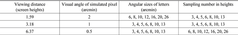
Letter Sizes in Experiment 2
The experiment consisted of one session containing all conditions, presented in random order. It took about two hours to complete.
Six subjects, 24 to 39 years old, participated. Three had participated in Experiment 1. All had normal or corrected-to-normal visual acuity and stereoacuity. If they would normally wear corrective lenses, they wore them during the experiment. All but one were naïve to the experimental purpose.
Figure 7 presents the effective resolutions for different conditions, averaged across subjects. The results were very consistent with those from Experiment 1. At 1.6 H and 3.2 H, temporal multiplexing provided significantly better resolution than either spatial-multiplexing method (
It has been argued that spatial multiplexing as implemented in many stereoscopic displays delivers effectively full-resolution binocular images, even though only half of the pixels are presented to each eye at a given time [2, 3]. We found no evidence to support this argument. At viewing distances of 1.6 and 3.2 H, the effective resolution with spatial multiplexing was
The fact that temporal multiplexing yielded greater resolution than spatial multiplexing at a distance of 3.2 H is significant, because this is the recommended viewing distance for HDTV [10]. However, many viewers tend to sit farther than the recommended distance, so they may experience less reduction in resolution with spatial multiplexing. Indeed, if they sit far enough, they will not experience a reduction at all.
Some previous studies had reported no loss in effective resolution for spatially interlaced TVs compared to temporally interlaced TVs, which is not the same as our finding. We think the most likely reason for the discrepancy is the visual stimuli that were used. Our experiment was designed to measure the threshold value for the two different stereoscopic presentation methods. Note that the subjects were able to score almost 100% when the letter size was larger than the thresholds for both presentation methods. It is possible that the previous studies had used stimuli that were easily recognizable on both presentation methods.
>
Implications for Ultra-High-Definition (UHD)
The resolution of Full HD was used because that was the prominent resolution format at the time. More recently, TV resolution has been transitioning to UHD. Despite the difference in resolution format, the experimental results and findings are applicable to formats with different resolutions, when converted into angular units at the eye. Visual resolution is determined in angular, not linear, units. This is why, for example, a person’s acuity is often stated in MAR (Minimum Angle of Resolution). Indeed, this is why the recommended viewing distance for a resolution format is determined from a calculation using angular units. 3.2 times screen height for HD and 1.6 times screen height for UHD both correspond to 60 pixels per degree [14]. Thus our results yield the same conclusion for HD and UHD: Spatial multiplexing will have lower effective resolution at the recommended viewing distance (3.2 and 1.6 H, respectively), though the difference will diminish at longer viewing distances.
>
Simulation of Appearance with Temporal and Spatial Multiplexing
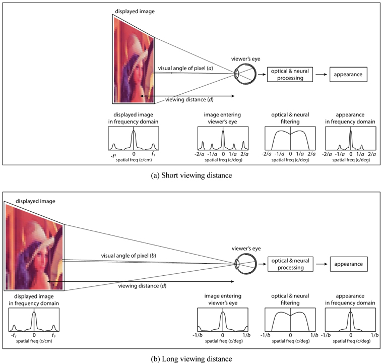
The early stages of vision involve low-pass filtering: the eye’s optics are aberrated, causing attenuation of high spatial frequencies; the photoreceptors are finite in size, also causing high-frequency attenuation; and photoreceptors are spatially pooled in many higher-order retinal neurons, producing further attenuation of high frequencies. Capturing and displaying a scene also involves low-pass filtering because of pixelation of sensors in capturing devices and pixelation of display panels. Because the visual process occurs after the display process, the percept derived from a display cannot have greater bandwidth than the direct percept. In other words, a display can at best maintain the bandwidth of direct observation.
Here we examine the pipeline from image capture/creation to image display to viewing in order to determine the expected appearance of images presented on temporally and spatially multiplexed displays for a typical viewer at difference distances. Figure 8 shows how the expected appearance will be affected by viewing distance: The upper and lower panels are for short and long viewing distances, respectively. The bottom graphics in each panel show how the image changes in the frequency domain through the pipeline of displaying and viewing. The process begins with the displayed images on the left. Here the units are cycles per distance on the display plane, so the amplitude spectra are identical because, whether viewed at short or long distance, they are the same physical size. The side lobes are aliases due to finite pixel size. At the eye, we express spatial frequency in angular units of cycles/degree because the low-pass filtering of early vision is to first approximation constant in those units. In angular units, the spectrum narrows and widens for short and long viewing distances, respectively. The image delivered to the eye then undergoes optical and neural filtering. We simulate this with the contrast sensitivity function (CSF) [15]. Specifically, we multiply the amplitude spectrum of the delivered image by the CSF to obtain the amplitude spectrum of the image after visual processing. The visual system behaves linearly near detection threshold and at high spatial frequencies (greater than 2 cycles/deg) [16], so we do not violate the linearity assumption by using the CSF in this way, because our goal is to determine when fine-detail artifacts will be just visible. In the resulting spectra the aliases remain at the short viewing distance, but are eliminated at the long distance. Thus, in this example, the display resolution is not high enough at short distance to avoid aliasing, but it is high enough at long distance.
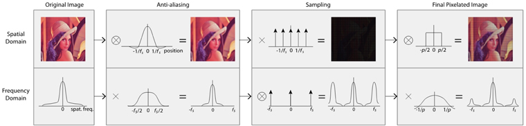
With an HD TV, temporal multiplexing delivers 56.5 pixels/deg at a viewing distance of 3 H. Spatial multiplexing delivers 56.5 pixels/deg horizontally, but only 29.3 pixels/deg vertically. To determine how appearance is likely to be affected in each of the two multiplexing techniques, we go through the procedure in Fig. 9.
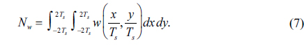
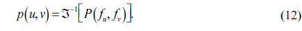
The intensity distribution function of the original image is

where

where ℑ is Fourier transformation and
where
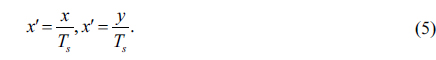
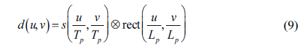
The intensity distribution of the antialiased image is then

where the normalization factor
We then sample the antialiased intensity distribution by multiplying the signal and an impulse train:
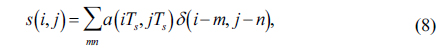
where
where

where
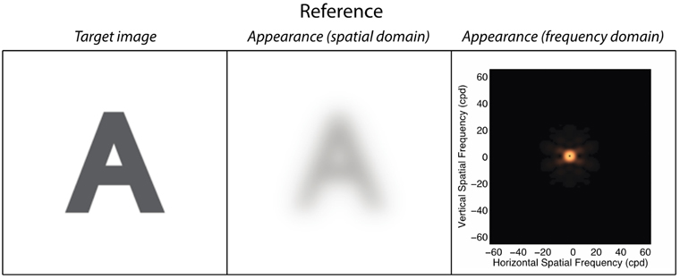
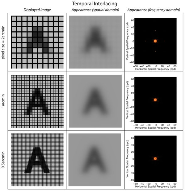
Using this procedure, we now compare temporal and spatial multiplexing at three viewing distances (1.6, 3.2, and 6.4 H, which yield respectively pixel sizes of 0.5, 1, and 2 arcmin). The target image is the letter ‘A’; its size is fixed at 10×8 arcmin for all viewing distances. Figure 10 shows how appearance is affected when the letter is directly viewed (
Figure 11 shows the simulation for temporal multiplexing for one eye. We halved the intensity of the target image to account for time multiplexing. From top to bottom, the viewing distances are 1.6, 3.2, and 6.4 H, corresponding to respective pixel sizes of 2, 1, and 0.5 arcmin. The fill factor
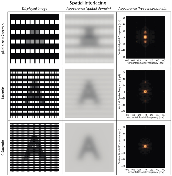
Figure 12 shows the simulation of spatial multiplexing for one eye. From left to right, the columns show the displayed image, its appearance in the spatial domain, and its appearance in the frequency domain. The appearance at viewing distances of 1.6 H and 3.2 H is notably poorer for spatial multiplexing than for temporal, due to the coarser vertical sampling. The pixel rows are more visible with spatial multiplexing, which is apparent in the right panels, where the vertical frequencies due to sampling are visible at the two shorter distances.
Our simulation shows how two widely used techniques for presenting stereoscopic imagery are likely to affect visual appearance. The simulations were done for one eye, so they do not necessarily inform us about appearance with binocular viewing, but our psychophysical results show quite clearly that effective resolution is lower with spatial multiplexing than with temporal multiplexing at short viewing distances. Those results are actually quite consistent with our simulations and suggest therefore that effective resolution can be well modeled by consideration of the monocular images.
We compared the effective resolutions of two stereoscopic 3D presentation methods, namely temporal multiplexing and spatial multiplexing. At short and medium viewing distances, temporal multiplexing provided greater effective resolution than spatial multiplexing. At long viewing distance, the two techniques provided similar resolution. The difference in resolution was significant at the recommended viewing distance for HD televisions.

![Three methods of stereo image presentation in spatial multiplexing [5, 6]. Same-line allocation uses the same rows from each eye’s image. Alternate-line allocation recruits rows from each eye’s image in an alternating fashion. Both-line allocation uses two rows from the left and right eyes’ images to generate one row in the stereo image.](http://oak.go.kr/repository/journal/21434/KGHHD@_2017_v1n1_34_f001.jpg)
![Stimuli for the visual acuity task. The stimuli followed the design criteria for the most widely used clinical visual acuity test [11]. Letter height was five times letter stroke width. Letter width was four times stroke width. Spacing between letters was two times letter width. Three randomly chosen letters were presented on each trial.](http://oak.go.kr/repository/journal/21434/KGHHD@_2017_v1n1_34_f002.jpg)