As described in the previous paper
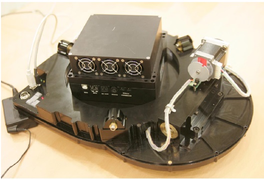
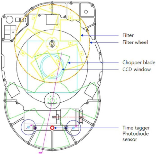
Optical wide-field patrol (OWL) has a detector subsystem consisting of a CCD camera, de-rotator, filter wheel, chopper and time tagger (Figs. 1 and 2). This mechanism makes it possible to produce multiple data points from observations of artificial satellites or space debris which moves faster than the sidereal rate of the background celestial objects. In the previous paper (Park et al. 2013), the development of a data reduction algorithm for this type of data was presented in detail. In this paper, the algorithm is reinvestigated and improved.
In Section 2, the previous reduction algorithm is summarized and a problem in the calculation of the streak length is raised. In Section 3, several similar studies are introduced. In Section 4, a method based on using the differential convolution mask is presented and Section 5 summarizes the paper.
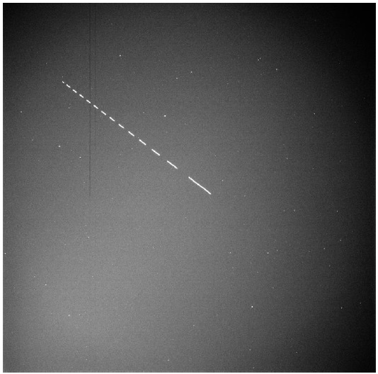
Fig. 3 is a sample of an OWL observation image. The reduction procedure in brief is as follows:
2.2 Streak Detection and Length Determination Using SExtractor
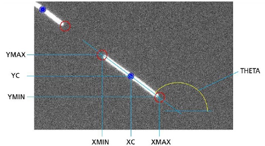
Photometry output using SExtractor includes various parameters such as position, magnitude, ellipticity, star/galaxy classification and coordinate of the rectangular region containing the detected object. Streak collection is performed using these parameters (ellipticity and star/galaxy classification). The collected streaks are aligned to a Legendre polynomial, usually as a straight line. Because it is clear that the length of a streak is proportional to the exposure time segment between obscurations by rotating chopper blades, defining the length of the streak is essential. In Park et al. (2013), this length value is determined using the coordinate values of the rectangular region containing the streak (Fig. 4) as follows:

2.3 Combining Positional Data with Time Log Data
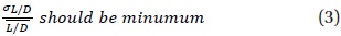
The chopper starts to rotate from a steady (stopped) state and the angular speed accelerates, making the length of the streak long at first but decreasing with time. The ratio of the line length (
In other words,

Adjusting the offset of the sequences of
2.4 Ambiguity of Length Determination
This reduction procedure requires an accurate streak length determination. But the streak length calculated simply from the diagonal of the rectangular region containing the streak cannot be measured directly. The pixel brightness begins to rise from the background when the chopper blade starts to open the CCD window, becomes half of the top value when the CCD window is half open (just when the blade edge hits the time tagger photodiode sensor at the opposite side of the CCD window), and reaches the top when the window is completely open. To measure the exact length of a streak, it is important to locate the endpoints of the streak accurately.
In the field of general image processing, just beyond the area of observational astronomy, there are various methods of feature detection based on mathematical calculations. Some of these methods are also adopted and studied for astronomical image analyses, including characterization of non star-like, elongated objects such as streaks.
3.1 Using “Tepui” Function as PSF
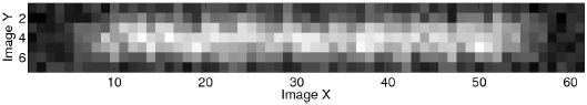
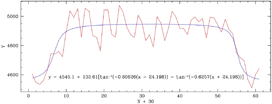
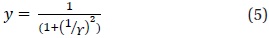
In Abad et al. (2004), an analytic function referred to as the “Tepui” function, Eq. (4) is used as a model profile of observed visual binary stars. Fig. 5 is a sample streak and Fig. 6 shows its “Tepui” fitting result. Abad et al. (2004) noted that the parameter “

Montojo et al. (2011) also suggested that streaks of artificial satellites fit to this “Tepui” function well along the
However, according to Abad et al. (2004), there must be additional fitting parameters to be calculated because the real observed streaks have rotation,
In 1988, Harris & Stephens (1988) suggested an edge detection algorithm based on image gradient. The underlying idea of this algorithm is that when a searching window with a box shape sweeps on an image, the sum of the pixel values inside the box does not change in a “flat” region in any direction, nor in an “edge” region along the edge direction, but changes significantly in all directions in the “corner” region. This idea can be implemented and parameterized easily using image pixel gradient. The Gaussian weighted (using
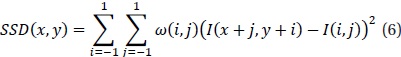
It can be expressed using the pixel gradients (

Hence, the squared sum is:
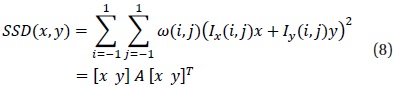
Where,
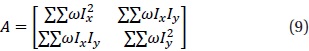
Finally, the response (

Where,
While Harris & Stephens (1988) tried to detect the features of objects using the gradient on the image plane, Kovesi (1999) presented another method using “phase congruency”. In this approach, regarding the image pattern as a linear sum of multiple signals, the phases (“

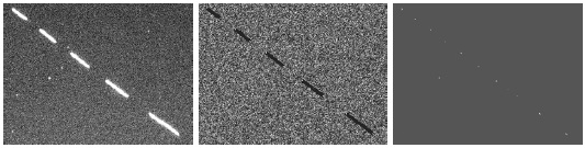
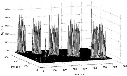
To calculate this for just a single image, several fast Fourier transform (FFT) and inverse FFTs are needed, resulting in excessive calculation time. Additionally, this calculation requires a specific study of the noise behavior of OWL observation images and parameter optimization, which can vary from image to image. Fig. 9 is a 3-dimensional plot of the phase congruency calculation result of Fig. 1. Because the noise model and parameter optimization are not complete, the endpoints of the streaks are not clearly defined.
4. REVISED REDUCTION ALGORITHM
4.1 “Differential” Convolution Mask
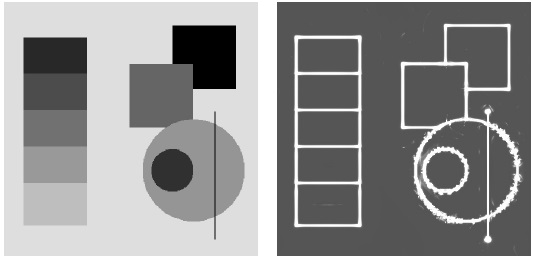
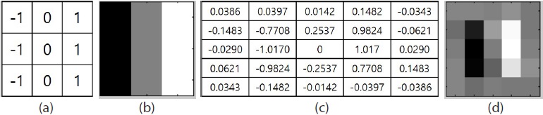
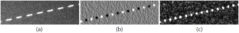
Prewitt (1970) presented a method of edge detection using a 3×3 convolution mask (Fig. 10(a)). The result of image convolution using this mask pattern as a convolution kernel is the horizontal image gradient of an input image because it calculates the difference of both sides of the central pixel. We hereafter refer to this mask pattern as the “differential” mask. Originally, Prewitt (1970) suggested using this mask in horizontal and vertical directions and calculating the Pythagorean root mean square to extract the feature pattern of objects in an image. But our purpose is not exactly the same and we can measure the position angle of the aligned streaks; the method (described in Section 4.2) is somewhat different. An example of the result is illustrated in Fig. 11. The input image (Fig. 11(a)) has streaks tilted 12.4˚ clockwise on it. The convolution mask (Figs. 10(a) and 10(b)) hence should also be rotated (Figs. 10(c) and 10(d)). After convolving using this rotated, bicubic-interpolated kernel, the rising and the declining positions of the streaks appear (Fig. 12(b)). Taking the absolute values of the convolved images shows us the endpoints of the streaks (Fig. 12(c)), where the absolute values of the image gradients are the most significant when the edges of the chopper blades obscure half of the CCD window as explained in Section 2.4.
4.2 Measuring the Lengths of Streaks and Making the Final Reduction Result
The procedure of measuring the lengths of streaks is as follows:
Because the newly identified endpoints are the direct observed points which the raw time log records correspond to, the number of the resultant data points is two times that of the case of Park et al. (2013), which considers only the center positions of the streaks.
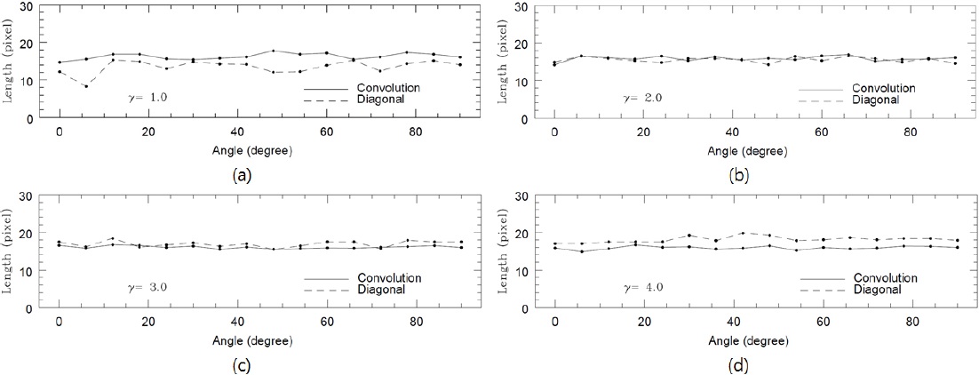
4.3 Comparison with the Old Method via Simulation
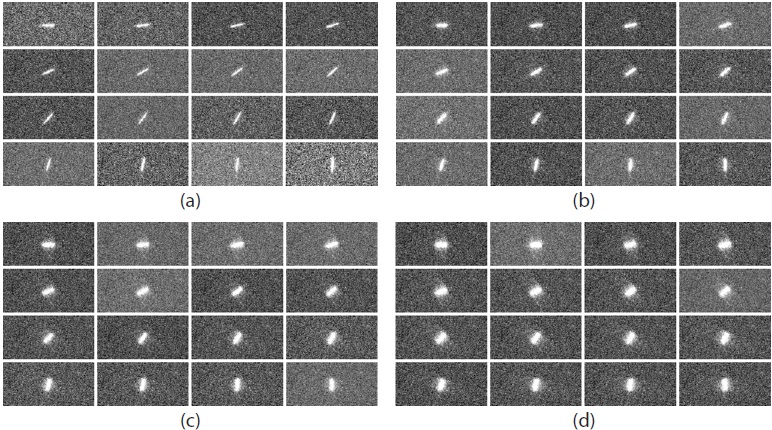
To compare the behaviors of the old and the new methods of streak length measurement, a brief simulation is performed using artificially created streak images. The streak model function is a “Tepui” function along the major axis and a Lorentzian profile along the minor axis as explained in Section 2.1, similar to the model in Montojo et al. (2011). The input parameters of the simulation are summarized in Table 1 and Fig. 12 shows images created using these parameters. The lengths of these streaks are calculated using the diagonal method of Park et al. (2013) and the convolution method. The results are shown in Fig. 13 for each
[Table 1.] Simulation parameters
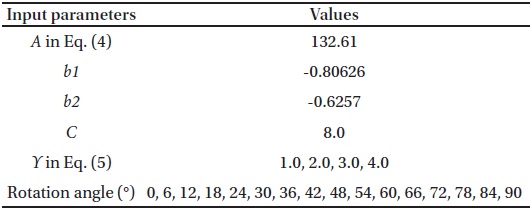
Simulation parameters
OWL is an automated observation and data acquisition system for fast moving objects such as artificial satellites and space debris near the Earth. It has a chopper system and a time tagger that can generate a large number of data points of the moving targets in a single observation. Park et al. (2013) reported a basic data reduction algorithm for this purpose based on the characteristic that the length of observed streak of a moving target trajectory cut by the chopper and the time durations of the exposures are proportional to each other. However, although an accurate measuring method of the lengths of the streaks is essential for this algorithm, the method used in the previous study was not accurate enough. In this paper, several related studies about feature detection in the field of image processing are examined and applied to the image data from OWL observation. The results demonstrate that the method of convolution using the “differential” mask pattern presented by Prewitt (1970) is a good solution. Using this, more exact results of streak length measurements are enabled, and the number of data points is increased up to two times enhancing the efficiency of the observation significantly.