The ionosphere, which is the layer of the atmosphere extending between 50 and several thousand kilometers above the Earth’s surface, produces different effects on Global Navigation Satellite Systems (GNSS) (Kintner & Ledvina 2005). The Total Electron Content (TEC), the total number of electrons integrated along the ray path from a Global Positioning System (GPS) satellite to a ground-based GPS receiver, is one of the most important ionospheric parameters because it directly affects the propagation of electromagnetic waves through the ionosphere.

Information on temporal and spatial variations in TEC is very useful for users of satellite-based navigation systems. Any changes in TEC are a serious concern, particularly at low and equatorial latitudes due to the strong variations in the ionosphere in this region. GPS based applications are widely used (Hofmann-Wellenhof et al. 2001) and they encounter largest errors as the result of free electrons in the path of the satellite signal (Klobuchar 1986). Therefore, variations in the GPS-TEC have been extensively studied (Maruyama et al. 2004).

Mapping the ionosphere is vital for various applications. The ionospheric map time series can be used to describe major ionospheric trends as a function of local time, season, and spatial location (Durmaz 2013). By analyzing these maps, ionospheric forecasting and broadcasting can be carried out and subsequently applied to many related applications.

By means of a large number of permanent tracking stations, GPS receivers can deliver large volumes of data suitable for continuous, near or real-time ionosphere monitoring during disturbed and quiet geomagnetic conditions, and thus offer an attractive alternative to traditional methods (e.g., the ionosonde network). Currently, GPS analysis centers generate Global Ionosphere Maps (GIM) on a daily basis. The widely-used GPS-derived GIMs provided by the International GPS Service (IGS) have a spatial resolution of 2.5° and 5.0° in latitude and longitude, respectively, and a 2 hr temporal resolution (Feltens & Jakowski 2002). Thus, although the IGS supports the scientific community with high-quality GPS products, the IGS GIMs cannot reproduce local, short-timescale processes in the ionosphere. In addition, the resolution of these products may not be sufficient to support high-quality GPS positioning, especially in the presence of local ionospheric disturbances. The need to produce high-resolution regional ionosphere models, supporting navigation, static positioning, and space weather research, is commonly recognized (Komjathy 1997; Hemtindez-Pajares et al. 1999). Even high-quality empirical ionosphere models do not provide sufficient accuracy to support all precise positioning applications, due to their insufficient temporal and spatial resolution (Grejner-Brzezinska et al. 2004, 2006).

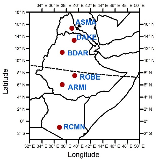
In this context, we investigate the suitability of twodimensional interpolation for mapping the East African region of the ionosphere using ground-based GPS receivers situated at Asmara, Mekelle, Bahir Dar, Robe, Arbaminch, and Nairobi. We have produced TEC maps with spatial resolution of 1°×1° latitude and longitude, respectively, and 2 hr temporal resolution, for the year 2008. The results show significant diurnal and seasonal dependence of the TEC.

TEC is an indicator of ionospheric variability derived from the modified GPS signal through a free-electron filled medium. It is also the ionospheric parameter that produces the greatest effect on GPS signals. GPS observations provide both carrier phase delay, L, and pseudorange, P, data for the dual frequency bands. GPS operates on two different frequencies, f₁ and f₂, which are derived from the fundamental frequency, f_o, of 10.23 MHz:

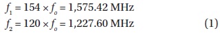
Both code and phase measurements are affected by the dispersive behavior of the ionosphere, but with different leading signs, resulting in delay between the two frequencies. This delay is characterized by the total electron content with the standard analysis method (Mannucci et al. 1998; Ciraolo et al. 2007). A dual-frequency GPS receiver can measure the difference in ionospheric delay between the L1 (1,575.42 MHz) and L2 (1,227.60 MHz) GPS frequencies, which are generally assumed to travel along the same ray path through the ionosphere. Thus, the relative group delay can be obtained by:

wher p₁ and p₂ ar the group path lengths corresponding to the high GPS frequency (f₁ = 1,575.42 MHz) and the low GPS frequency (f₂ = 1,227.6 MHz), respectively. Thus, TEC can be obtained from the measurement of p₁ − p₂ using equation (2). TEC can be expressed in Total Electron Content Units (TECU), where 1 TECU=1×10¹⁶ electrons m^-2.

The TEC obtained from equation (2) is determined along the line of sight between a GPS satellite and receiver, known as Slant TEC (STEC). STEC can be converted to Vertical TEC (VTEC) at the Ionospheric Pierce Point (IPP) by applying the ionospheric thin shell model (Mannucci et al. 1998). The relationship between STEC and VTEC is given in terms of the zenith angle at the IPP, χ’, and the zenith angle at the receiver position, χ, as follows:

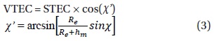
where R_e is the radius of the Earth, and h_m is the height of the ionospheric layer, assumed here to be 350 km.

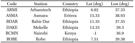
For this study, we used GPS-TEC data acquired during the year 2008. The GPS-TEC data were obtained from dual-frequency GPS receivers located in East Africa, as shown in Fig. 1 with their geographic coordinates listed in Table 1. The VTEC values were calculated using the method explained above (Ciraolo et al. 2007).

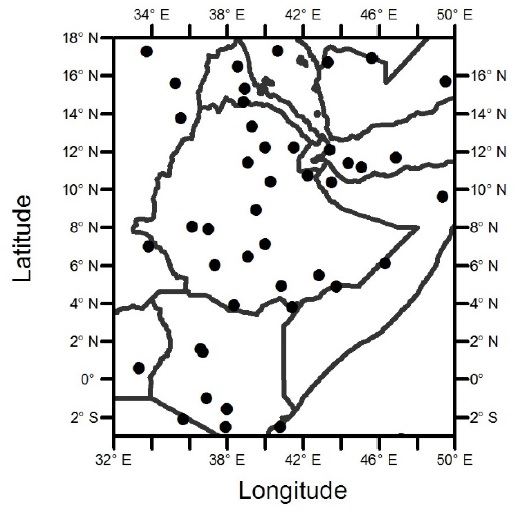
Fig. 2 shows the distribution of IPPs in East Africa at 0600 UT on October 3, 2008. Each calculated VTEC value is then projected on to the corresponding IPP to represent the ionosphere at those points. Noting that the VTEC points are not uniformly distributed, we adopted an Inverse Distance Weighted (IDW) interpolation of VTEC to map the ionosphere across the region.

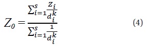
The IDW interpolation is an exact method that enforces the condition that the estimated value of a point is influenced more by nearby known points than by those farther away. The general equation for the IDW method is:

wjere Z₀ is the estimated value at point 0, Z_i is the Z value at known point i, d_i is the distance between point i and point 0, s is the number of known points used in the estimation, and k is the specified power. Using the IPPs with their corresponding VTEC, we applied the IDW interpolation scheme to calculate the VTEC values within 1° × 1° grid squares.

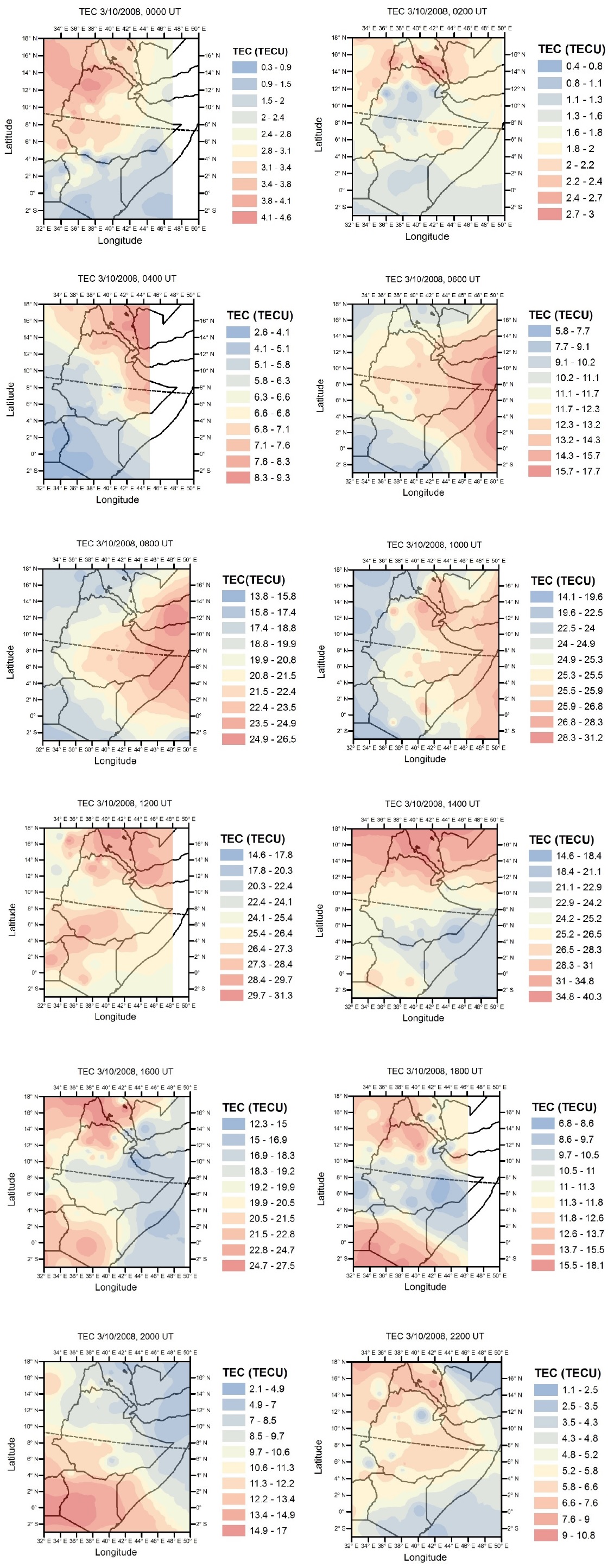
Fig. 3 illustrates how VTEC values vary over a typical day in East Africa. The figure shows VTEC maps of the East African ionosphere in 2 hr intervals from 0000–2200 UT on October 3, 2008. The maps generated at 1000 UT, 1200 UT, and 1400 UT (1300 LT, 1500 LT, and 1700 LT) indicate that the VTEC values are higher in the afternoon than during other times of the day. This is probably because the eastward electric field becomes strong in the afternoon and causes enhancement of equatorial ionization anomaly, resulting in higher ionospheric electron densities at low latitudes (and hence, higher VTEC values). Pi et al. (2003) have shown that the enhancement of E×B drift often occurs in the afternoon.

Fig. 3 shows that during the early hours of the day, beginning at 0400 UT, while the sun is still rising the VTEC values slowly increase from the night time value. During the evening hours, the sun is setting and the VTEC values therefore gradually reduce, which can be seen in the maps generated at 1400 UT and 1600 UT. After sunset, VTEC values rapidly decrease due to the electron recombination process in the absence of ionizing solar UV, as shown in the maps generated at 1800 UT, 2000 UT, 2200 UT, 0000 UT, and 0200 UT.

The equatorial and low latitude ionosphere is known to have one of the most important dynamic features. It is characterized by the Equatorial Ionization Anomaly (EIA), which has a unique structure comprising two ionization peaks at about ±17° latitude on each side of the magnetic equator with a trough in ionization between them (Appleton 1954). In Fig. 3, the equatorial anomaly is apparent in both the northern and southern hemispheres, compared to the magnetic equator, at 1200 UT, 1400 UT, and 1600 UT, with a maximum difference at 1400 UT.

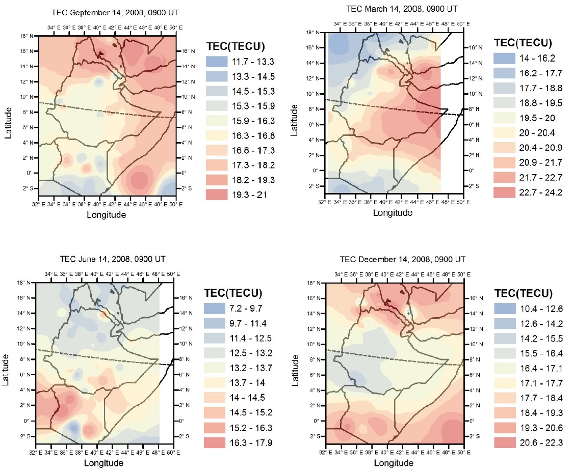
The intensity of solar radiation reaching the ionosphere changes with the seasons of the year. Fig. 4 illustrates the variations in the East African ionosphere during the four seasons of 2008. The VTEC maps in Fig. 4 are shown for March 15, June 15, September 15, and December 15, respectively, which were chosen to represent a typical day in spring, summer, fall, and winter. The displayed maps were generated at 0900 UT (1200 LT) for each of the selected dates.

As discussed by Tsai et al. (2001), the subsolar point is close to the magnetic equator during the summer northern hemisphere. Due to this effect the trans-equatorial neutral wind suppresses the northern equatorial ionization anomaly and plasma is concentrated in the southern anomaly. This phenomenon is clearly visible in Fig. 4 during the June solstice. On the other hand, during the summer southern hemisphere, the subsolar point is located far from the magnetic equator. As a result, the trans-equatorial wind is too weak to transport plasma to the northern hemisphere and thus sustains the equatorial ionization anomaly at both sides of the equator, as shown in Fig. 4 during the December solstice. During the two equinoxes the subsolar point is located directly over the equator, which increases ionization and therefore causes high TECs in this region. This is related to the so-called semi-annual anomaly, where the peak TEC occurs during the equinoctial months in most regions (Yu et al. 2006).

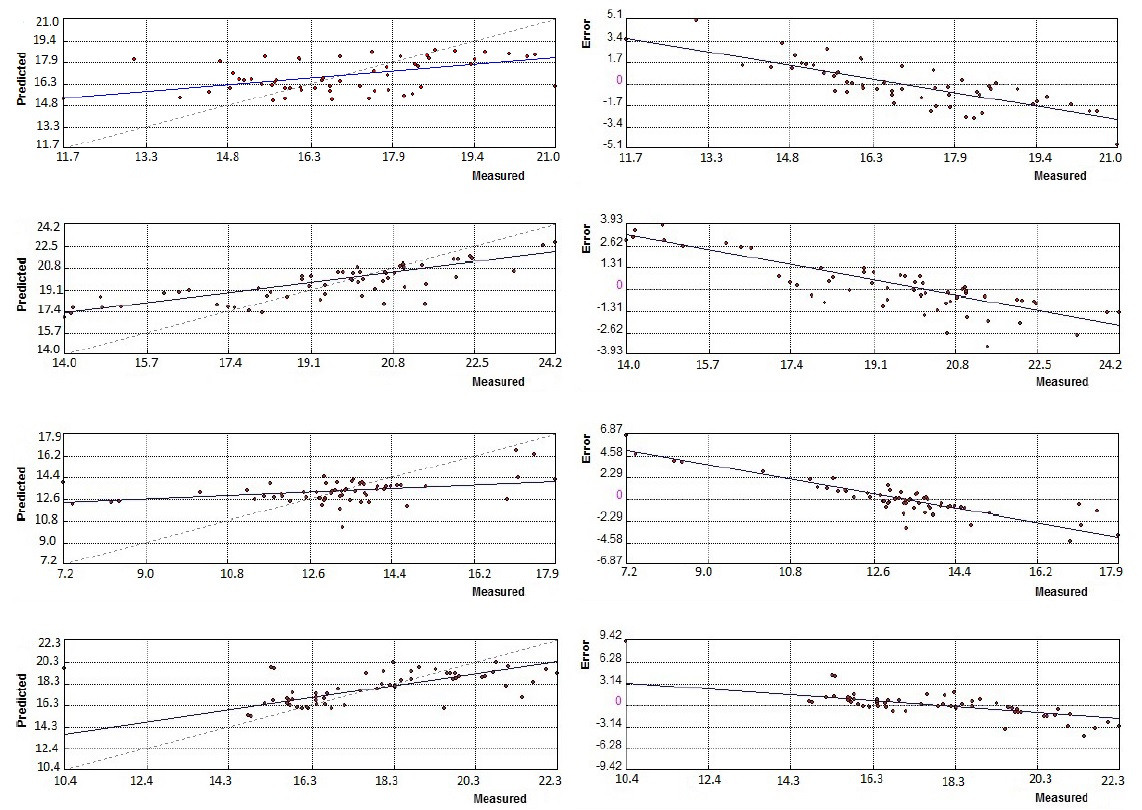
We use a cross-validation technique to evaluate the performance of our interpolated ionospheric map. This method removes each data location one at a time and compares the measured value with the interpolated value at that location. The comparison between the measured and interpolated VTEC is shown in Fig. 5. The interpolated VTEC has a maximum mean error (difference between the interpolated and measured values) of 0.20 TECU (10¹⁶ m^-2) in March and a minimum mean error of 0.04 TECU in September. The maximum and minimum errors of 9.42 and 3.93 TECU occurred in December and March, respectively. It is apparent from Fig. 5 that the interpolated values tend to be larger and smaller than the measured values toward the low and high ends of the measured TEC. This characteristic is unavoidable because the interpolation method always calculates values within the range of measured values used.

A regional ionospheric VTEC map for East Africa in 2008 has been constructed to study the temporal, spatial, and seasonal variations in the equatorial ionosphere using ground-based GPS data. The VTEC map shows the apparent diurnal variation in temporal and spatial manners. The map also exhibits an equatorial ionospheric anomaly, characterized by low VTEC around the equator and high VTEC in both subtropical regions. We noted that the equatorial anomaly is asymmetric during the June solstice, due to the strong trans-equatorial neutral wind. We also identified the semi-annual ionospheric anomaly, where the maximum VTECs are observed during the equinoxes. We demonstrated the reliability of the map by comparing the measured VTEC with the interpolated VTEC over the region, showing a mean error (difference between the measured and interpolated values) range of 0.04–0.2 TECU. In the future we anticipate that this type of TEC map will be improved with additional measured TEC values, and thus can be used to study the equatorial ionosphere of the African sector where very few monitoring facilities are currently available.