The focal length (FL) of an imaging optical system is a fundamental characteristic, and many methods have been proposed [1-3] for the accurate determination of FL. Because FL is defined for an ideal system, most of the methods face uncertainties due to aberrations of the physical systems, as well as the measurements of the system. In contrast, the method utilized by Moiré interferometry is different; measurements usually take place near the optical system and far from the focal plane, and the effect of the aberration can be minimal or negligible in most cases. Thus this method is commonly used for examining long focal lengths [4-6].

When a converging beam is incident upon a periodic transmission grating, the (de)magnified self-image of the grating is formed at regular distances, the so-called Talbot distance, from the grating. The (de)magnification, which depends on the convergence of the beam and on the distance away from the grating, is the key aspect for the determination of the focal distance of the lens. To determine the (de)magnification, a second grating is typically placed at the (de)magnified image of the first grating, to form a superimposed pattern of the two gratings, the so-called Moiré fringe. The second grating is usually rotated a small angle with respect to the first, and the angle between the gratings affects the Moiré fringe as a whole. Thus, accurate information on the angle between the gratings is as important as analyzing the fringe accurately.

L. M. Sanchez-Brea et al. [7] recently demonstrated that the period of one self-image produced by a grating can be used for beam collimation, which has been achieved by Moiré interferometry with double-grating imaging [8]. S. Lee also recently used the numerical simulations with the Fresnel diffraction integral to demonstrate the determination of focal length of a lens without Moiré fringes [9]. The necessary condition for the determination was the usage of the original Fourier transform for the precise spatial frequency resolution beyond the limited frequency interval determined by the conventional fast Fourier transform analysis. Despite the calculation of the accurate spectral frequency to analyze the Talbot self-images, the period of the grating still remained in the uncertainty range of a few percent given by the manufacturer [10], which left the final focal distance determinations with the same uncertainty. The simplification of using one grating only, however, provides a condition to determine the focal distance without a priori knowledge of the period of the grating. A linear relation between the (de)magnified periods of the Talbot images and the lens-to-grating distance can circumvent the requirement of the period of the grating.

The proposed method will be presented in two parts of an experiment: a preliminary collimation test on the incident light, and the main part: the focal distance determination of a thick lens whose effective focal length is 500 mm.

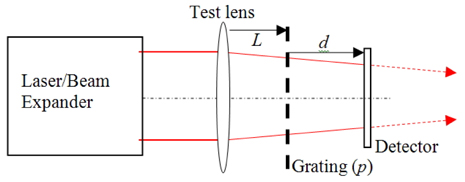
Figure 1 shows the schematic layout of the setup, in which a positive lens causes a beam to converge as it propagates through a binary grating with period of p, onto a detector. The grating is located at an arbitrary distance, L, from the back surface of the lens and the detector is located at the distance, d, from the grating, where a (de)magnified image of the grating is measured.

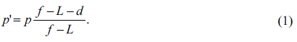
The (de)magnified period of the grating, p', at the detector can be computed by using similar triangle properties, with the help of Fig. 1, to be

The f is the focal distance measured from the back surface of the lens to the focal point, which will be used differently in this paper from the focal length of the lens. If a collimated beam is incident to the lens, the focal distance becomes the back focal length. Here the distance d would be called the Talbot distance if the beam were collimated. For converging or diverging beams, the Talbot distance would be slightly modified [4]. It is important to have a sharp (de)magnified-image to form an optimal image with an accurate measurement of the distance between the grating and detector for the focal distance determination. With the measured (de)magnification, p' / p, the focal distance can be expressed as

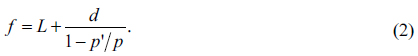
While the (de)magnified period can be determined accurately by analyzing the frequency spectrum of the Talbot image using the original Fourier transform described below, the period of the grating is usually provided by the manufacturer with some stated uncertainty. Measuring the period of the grating with enough accuracy could be a separate project. Thus, we propose an approximate method to circumvent the requirement of the period of the grating.

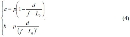
Let us imagine a set of measurements of the (de)magnified period as a function of the distance L, which is varied as L₀+L_x, where L_x is the small variation around the initial value of L₀, while the distance d remains constant. Then, Eq. (1) can be approximated as a linear function as expressed as

and the intercept and slope of the linear function can be given by

If the intercept is divided by the slope, the result becomes independent of the period of the grating as

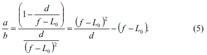
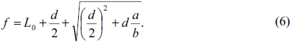
Eq. (5) can be recognized as a quadratic equation for the variable (f−L₀) and the focal distance can be determined from the solution of

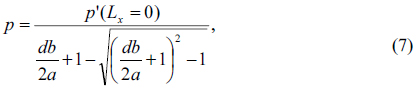
Thus, a set of (de)magnified period measurements with the variation of the distance between the lens and grating can enable us to determine the focal distance of the system under test without the original period of the grating. The original period of the grating can also be computed from the measurements by substituting Eq. (6) into Eq. (1) as

which can be confirmed by comparison with the nominal value and the manufacturer’s tolerance.

A set of specifications of the system used in the experiment is as follows. The test lens is a plano-convex lens (Rolyn optics, f=500 mm, D=90 mm, center thickness=6.6 mm), whose flat side is toward the grating, and the (de)magnified images of a binary (50% duty cycle) transmission grating (Edmund optics, #58-775) were measured with a digital camera (Point Grey Flea 2). The resolution of each image is 1032 × 776 pixels and the pixel size is 4.65 × 4.65 μm² . The gain and shutter time of the camera were adjusted so that the image is overall under the saturation level. The experiment consists of two parts: preliminary and main part.

The preliminary part is to check the collimation of the incident beam (λ=0.6328 μm) to the test lens after a beam expander. A shear plate was used to verify collimation during setup, and a second check is described here. The beam passed through the grating and illuminated the camera without the test lens. The Talbot distance is calculated as 15.8 mm for the combination of the period and wavelength of the light. However, this image plane is inside the camera; the distance from the camera flange to the image plane is 17.99 mm according to the dimensional drawing provided by the manufacturer, and a gap from the grating to the camera opening was needed for the alignment of the setup. Thus, the distance from the grating to the image plane was adjusted to view an optimal image for the analysis, and it was 20.22 mm for this preliminary measurement. The distance from the beam expander to the grating was 56.34 mm. The (de)magnified period was determined as 0.1000 mm with the method described below. With the period of the grating assumed as 0.1 mm, the focal distance of the collimated beam can be determined as about 5 km, which can certainly be regarded as infinite for the test lens.

Once the collimation of the beam was confirmed, the main part of the experiment was performed with the test lens being inserted between the beam expander and grating. The distance L₀ from the lens to the grating was varied from 56.34 mm (L_x= −10 mm) to 76.34 mm (L_x=10 mm) with the interval of 2 mm while the distance d from the grating to the image plane was fixed at 26.51 mm. The same grating and detector were used. Figure 2 shows the Talbot image measured for the L₀ of 66.34 mm (L_x=0 mm). The period can be estimated based on the number of vertical dark lines, and there are roughly 51 lines, which correspond to the period of about 0.094 mm, less than 0.1 mm, indicating a converging beam, as expected.

The lens, in a self-centering mount, was attached to the optical table. The camera, and the grating in a rotation mount, were mounted on a translation stage with a resolution of 0.01 mm. Gage pins were used to measure the grating-to-camera flange distance to better than 0.01 mm, while avoiding scratching and allowing adjustments for parallelism between the two faces.

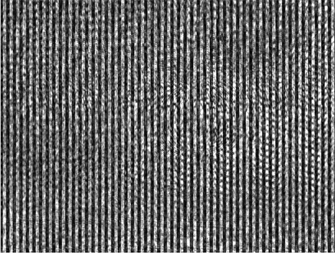
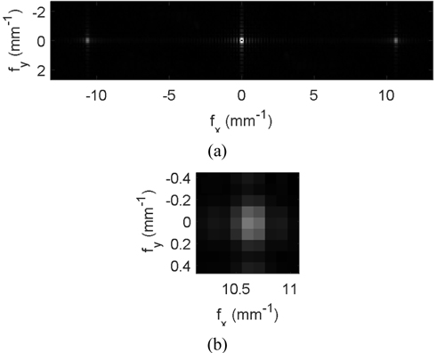
Figure 3 shows the frequency spectrum calculated by the fast Fourier transform (FFT) for the image shown in Fig. 2. To use the FFT, an image array of 2048 × 2048 pixels was used, with the original image (1032, 776 pixels) being embedded inside the array and the rest of it being set as zeros. An image array of 1024 × 1024 could be used to reduce the analyzing time, but this array reduces the frequency precision by a half, too. Because the size of each pixel is 4.65 μm, the physical dimension of the array for the FFT becomes 9.5232 mm and the spatial frequency interval corresponding to each pixel in the spectrum can be computed as 0.105 (=1/9.5232) mm^-1 . The frequency spectrum at the origin is the sum of all the pixels’ intensities, and the rest of the spectrum becomes almost zero if the spectrum is normalized to it. Thus, the spatial frequency point corresponding to 0 mm^-1 was set to zero, and the rest of the spectrum was normalized in intensity to fit into an 8-bit grayscale (with 256 grays) with black (white) being the minimum (maximum) intensity. Only a partial spectrum (51, 251 pixels) centered on the origin is shown in Fig. 3(a), and Fig. 3(b) shows the magnified spectrum centered at the spectral peak at about 10.6 mm^-1 . The spectral peak is located at a pixel offset of (101, 0) or (-101, 0) from the origin, and the (de)magnified period is 0.094289 mm (=9.5232/101). If the (de)magnified period is substituted into Eq. (2), the focal length of the lens becomes 530.5 mm, which is 30.5 mm more than the expected value.

The frequency interval with the FFT can be shortened in half by doubling the image array, and the frequency spectrum will become doubly dense with the expense of execution time of 4 times. Doubling a number of times causes the execution time to be exponentially increasing. To take an advantage of the FFT without the expense of the execution time, a set of analyzing procedures [9], which is composed of the original Fourier transforms, was performed for the frequency spectrum calculated by the FFT: 1) a square region of the spectrum centered on the spectral peak is divided into a 5-by-5 grid of frequency components, 2) the spectra for the frequency components are calculated with the original Fourier transform, 3) among the 25 spectra, the maximum component is sought and found, 4) a new square region, which is centered on the new component and has a side length that is half that of the previous region, is subdivided again, and 5) the searching procedure is repeated a number of times. The frequency of the spectral peak was finally calculated as a center-of-intensity among the last 25 spectra.

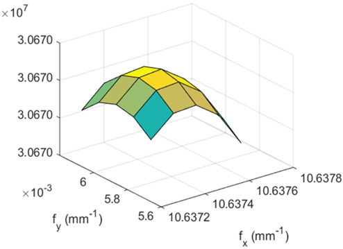
Figure 4 shows the surface plot for the 25 spectra after 9 iterations of the procedure. The uncertainty of the frequency analysis is then 0.0001 (=0.105/210) mm^-1 . The plot shows a well-determined peak at (10.6375, 0.0059) mm^-1 . The inverse of the distance of the spectral peak from the origin gives the (de)magnified period as 0.094007 mm, and the rulings are -0.03° from the vertical line of the image array. A similar value for the angle was observed during the main part of the experiment. With the period of 0.1 mm of the grating, the focal distance can be calculated as 508.7 mm by Eq. (2), which is 8.7 mm more than the expected value.

The difference of 8.7 mm, about 1.7% in accuracy, can be regarded as small enough. But it was calculated based on the condition that the period of the grating is 0.1 mm. If the period was changed from 0.1 mm to 0.0999 mm by 0.1%, the focal distance would be 515.7 mm. The difference becomes 15.7 mm, about twice the error. Thus, the determined focal distance is still uncertain unless the period of the grating is known accurately. This demonstrates the importance of the accurate determination of the period of the grating.

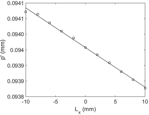
Figure 5 shows the set of the (de)magnified periods with the variation of the distance from the lens to the grating. They were fitted to a linear function and the slope and intercept were used to calculate the trend line, which is also shown in Fig. 5. The determined (de)magnified periods agree well with the line with negligible differences, which clearly validates the proposed method and the accompanying theory. The focal distance and the original period of the grating can be determined with Eq. (6) and Eq. (7), and they are 522.7 mm and 0.0998 mm, respectively. In a glance, the determined focal distance seems worse than the value calculated from a grating period of 0.1 mm. But substitution of the determined period of the grating of 0.0998 mm, from the Talbot image measured in collimated light, can explain the apparent error.

The newly calculated period of the grating, 0.0998 mm, which is 0.2% below the manufacturer’s value, is smaller than the (de)magnified period, 0.1000 mm, measured during the preliminary collimation checkup, and the corresponding focal distance of the collimated light needs to be changed from 5 km to -10,059 mm, meaning that the incident beam is diverging. Thus, lens illumination with a diverging, not parallel, beam needs to be considered. The object distance to the lens is then 10,059 mm, not infinite, and the corresponding image distance becomes 526.2 mm from this lens whose effective focal length is 500 mm.

Having considered the fact that the Talbot effect is the result of a periodic structure illuminated by a converging beam, the light after the lens with the image distance of 526.2 mm corresponds to the converging beam with the focal distance of 526.2 mm. That is, the determined focal distance of 522.7 mm must be compared with the 526.2 mm, not 500 mm, and the difference becomes 3.5 mm short. Furthermore, the distance 522.7 mm was from the vertex of the flat side of the lens to the image point, while the distance 526.2 mm was from the secondary principal plane to the image point, so the distance from the vertex to the secondary principal plane, 4.3 mm (=6.6 mm/1.52) must be subtracted from 526.2 mm to compare both values with each other. The difference becomes 0.8 mm, which is 0.15% more than the nominal value of 521.9 mm. Because the beam expander has no adjustment, no further test with the incident beam was performed.

Because the nominal focal length of the test lens has a tolerance of a few percent, the stated error of 0.15% for the focal distance of 521.9 mm might not be appropriate, but the set of measurements demonstrated the validity of our proposed method for focal distance measurements for both single lenses and optical systems. The precision of the method is subject to further studies.

We present a simple method for determining the focal distance with Talbot self-images with one grating. This method does not even require an accurate grating period. A linear relation between the (de)magnified periods of the Talbot images and the lens-to-grating distance was used to determine the focal distance of the converging beam within 0.15% for a lens whose nominal focal distance is 521.9 mm. The period of the grating was also determined to be 0.2% short of the nominal value of 0.1 mm.