The performance of a staring infrared imaging system can be characterized based on estimating the modulation transfer function (MTF). The slant edge method is a widely used MTF estimation method, which can effectively solve the aliasing problem caused by the discrete undersampling of the infrared focal plane array. However, the traditional slant edge method has some limitations such as the low precision of the edge angle extraction and using the approximate function to fit the edge spread function (ESF), which affects the accuracy of the MTF estimation. In this paper, we propose a modified slant edge method, including an edge angle extraction method that can improve the precision of the edge angle extraction and an ESF fitting algorithm which is based on the transfer function model of the imaging system, to enhance the accuracy of the MTF estimation. This modified slant edge method presents higher estimation accuracy and better immunity to noise and edge angle than other traditional methods, which is demonstrated by the simulation and application experiments operated in our study.
With the staring infrared imaging systems becoming more widely used, the accurate imaging quality assessment of infrared imaging systems is becoming more necessary and important. The imaging quality of an infrared imaging system is generally evaluated by the modulation transfer function (MTF) [1-3]. MTF is the magnitude of the optical transfer function (OTF), which is the Fourier Transform of the response of the imaging system to a point source (PSF). For digital imaging devices, the sample is discrete and inadequate, which causes the aliasing of the system. The aliasing problem and noise will make it more difficult to accurately estimate the MTF, therefore they must be eliminated in MTF estimation.
Nowadays, the estimation of the MTF of an imaging system has two major methods including the fixed targets method and the random targets method. The fixed targets method generally utilizes the slit target and knife edge target [4]. The random targets method often uses the random targets with known spatial frequency details [5]. Chambliss
The slant edge method measures the MTF from the image of the knife edge target [8]. This method is an effective and well-known method, which has been specified in ISO Standard 12233 [9]. The process of the slant edge method is simple and effective, and the manufacture of the knife edge target is very easy. However, some limitations still affect the accuracy of the MTF estimation in the slant edge method. Firstly, the edge angle cannot be extracted accurately from the image of the knife edge target with noise, which affects the projection direction of the pixels in the knife edge image [10]. Secondly, the ESF fitting is based on the approximate functions, such as the error function proposed by Bentzen [11], the sum of a Gaussian and an exponential function proposed by Yin [12], and the Fermi function proposed by Tzannes [1], which is based on the fact that their shapes are similar to the shape of the ESF. Therefore, the accuracy of the MTF estimation will be affected by these reasons.
In this paper, we analyze the influence of the edge angle extraction and the ESF fitting on the accuracy of the MTF estimation and propose a modified slant edge method. In this method, a new edge angle extraction method is proposed to improve the accuracy of the edge angle extraction. The ESF fitting method is built based on the transfer function model of the imaging system. It differs from the approximate function fitting in theory and has a higher accuracy. The accuracy of the MTF estimation is improved by the modified slant edge method.
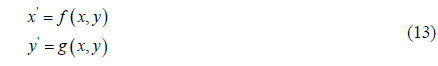
Given that the optical imaging system can be considered as a linear system, the relationship between the object and the image can be expressed as in Eq. (1):

where

When the object is a point source, the MTF can be deduced from Eqs. (1) and (2):

The line spread function (LSF) can be taken as a 1-D PSF [8], as shown in Eq. (4):

Based on Eq. (4), the 1-D MTF can be deduced from the LSF, as shown in Eq. (5):

In the case of the slant edge method, the object is the knife edge target which can be expressed by the Heaviside function, as shown in Eq. (6):

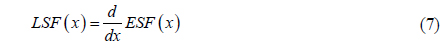
The LSF can be deduced from calculating the derivative of the ESF which is the response of the imaging system to the knife edge target. The relationship is expressed as in Eq. (7):
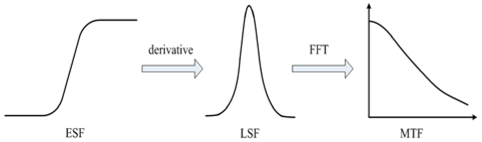
Based on the previously mentioned eqs., the MTF of the imaging system can be estimated by extracting the ESF from the image of the knife edge target. This process can be illustrated as shown in Fig. 1.
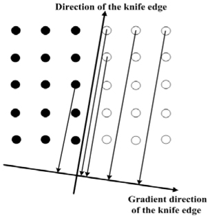
In the ISO Standard 12233 [9], the slant edge method has been described in detail. The knife edge must be slightly slanted to the horizontal or vertical direction of the focal plane array, which can effectively increase the sampling rate and eliminate the aliasing problem. The knife edge position in every data line is estimated by calculating the derivative of the discrete data, and determining the centroid as the knife edge position at a sub-pixel position. Through the estimated knife edge positions, a linear regression is used to estimate the edge angle, after which the pixels in the knife edge area are projected onto the gradient direction of the knife edge, as shown in Fig. 2. Then, a discrete ESF can be acquired to estimate the MTF.
There are two commonly used methods for dealing with the discrete ESF for estimating the MTF. One method utilized in the ISO Standard 12233 is to divide the gradient direction of the knife edge into bins with the width equal to a quarter of the origin sampling interval and average the gray values of the pixels in the same bin. Then, the discrete ESF with the equal sampling interval is obtained to estimate the MTF. Another method proposed in many studies is to fit the discrete ESF by the approximate functions as mentioned in Section I, which is based on the fact that their shapes are similar to the shape of the ESF.
Based on the previous discussion, the widely used traditional slant edge methods still have some problems, which make the MTF estimation inaccurate. Firstly, it is sensitive to the noise, because the edge angle is estimated by taking the derivative of every data line. If the edge angle extraction is inaccurate, the acquired ESF will deviate from the ideal ESF, which affects the accuracy of the MTF estimation. Secondly, when applying the discrete and equal sampling interval ESF to calculate the MTF, it will amplify the influence of the noise on estimating the MTF, as shown in Eqs. (8) and (9):

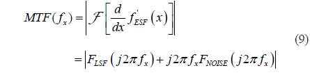
Where
In order to solve these problems and improve the accuracy of the MTF estimation, this paper proposes a modified slant edge method to improve the accuracy of the edge angle extraction and the discrete ESF fitting.
III. MODIFIED SLANT EDGE METHOD
The slant edge method estimates the MTF by analyzing a rectangular region of interest (ROI) in the image of the knife edge target acquired by the infrared imaging system. The ROI including the slant edge is chosen by the user. In the traditional slant edge method, every data line in the ROI is taken the derivative, and estimating the centroid position, which is equal to the knife edge position in every data line, and operating a linear regression to estimate the edge angle. This method is easily affected by the noise, because all data in the ROI need to have its derivative taken and the linear regression also has errors. This section proposes a new method for the edge angle extraction.
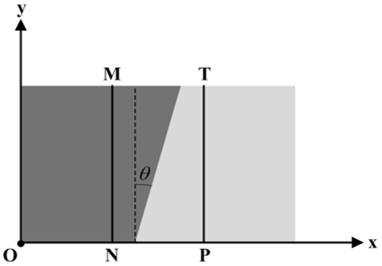
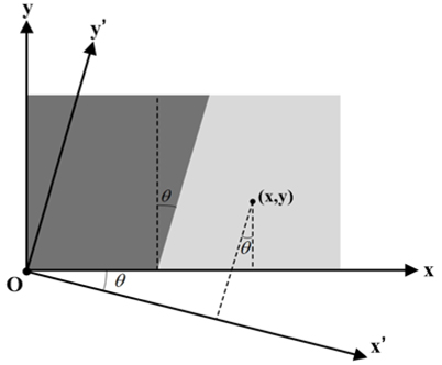
The ROI of the image of the knife edge target is illustrated as shown in Fig. 3. A 2-D coordinate is built where the x-axis and y-axis are set along the horizontal and vertical directions of the ROI, and the origin is set at the point O. The edge angle
The process of the edge angle extraction can be summarized as follows:
Firstly, the x-coordinates of the pixels in the ROI are used to determine whether the pixels are in the region for estimating the edge angle, as shown in Eq. (10):

If the pixels in the ROI satisfy Eq. (10), they are in the region for the edge angle estimation.
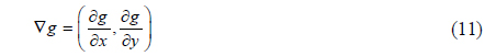
Secondly, the gradient operator is used to deal with the pixels in this region, as shown in Eq. (11):

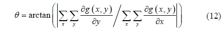
Then, the statistical gradient direction of the knife edge can be obtained from Eq. (12), which is equal to the edge angle.

Where
Finally, after the edge angle is extracted, all the pixels in the ROI can be projected onto the gradient direction of the knife edge to obtain the discrete ESF. A new 2-D coordinate
Where

Then Eq. (14) can be simplified to deduce the final conversion function of the coordinate, which is as shown in Eq. (15):

This new method of the edge angle extraction only needs to utilize a small user-defined region in the ROI, because the other regions away from the knife edge do not affect the edge angle estimation, using the small region to estimate the edge angle can decrease the influence of noise, which appears in other regions. The calculation of the edge angle uses the statistical method by analyzing the gradient of the pixels. Therefore, the new method is more robust against noise than the traditional slant edge method.
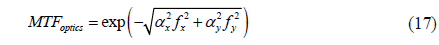
After projecting the pixels onto the gradient direction of the knife edge, the discrete ESF is obtained, and there are two methods that have been described in Section II for dealing with the discrete ESF to estimate the MTF along the gradient direction of the knife edge. The disadvantages of the two methods also have been introduced. In this section, a new ESF estimation method is built based on the transfer function model of the infrared imaging system. The transfer functions can be expressed as the following functions:
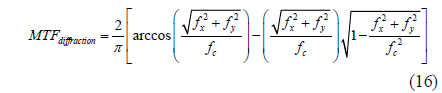


Where
The MTF estimation uses the 1-D transfer function model. The

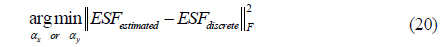
The adequate
IV. SIMULATION AND APPLICATION EXPERIMENTS
In order to verify the feasibility and validity of the modified slant edge method, a simulation experiment and an application experiment of testing MWIR imaging system were performed in this study. The modified slant edge method (MSEM) was compared with the ISO 12233 slant edge method and the traditional slant edge method (TSEM). For the TSEM, the edge angle extraction method is same with the ISO 12233 method, and the ESF fitting method utilizes the Fermi function, which is generally used in other studies.
A simulation experiment is designed to analyze the accuracy and stability of the edge angle extraction and the MTF estimation of the previously mentioned methods. For the edge angle extraction method in the ISO 12233 method and TSEM, a method combined differentiation calculation with linear regression is used, which is called the traditional edge angle extraction method (TEAEM).
The design details of the simulation experiment are illuminated as follows:
Firstly, an ideal image of the knife edge is built, and the convolution operation between the ideal image and a known PSF is performed to simulate the real infrared imaging system. The PSF is denoted as a Gaussian function, and the theoretic MTF curve can be acquired by Eq. (3).
Secondly, white noises are joined in the simulated image to analyze the influence of noise on the edge angle extraction and the MTF estimation.
Finally, we generate some simulated images with various edge angles and with various SNRs. These simulated images are analyzed by the different methods. For analyzing every simulated image, the simulated image is the ROI of each method to estimate the MTF. Therefore, the same analysis condition of each method can guarantee the validity of the comparison experiment. A simulated image of the knife edge with edge angle of 10° and with SNR of 40 dB is shown in Fig. 5.
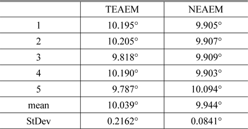
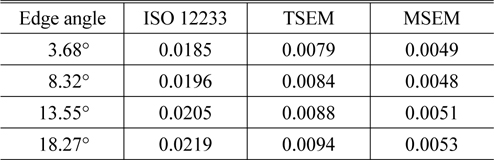
The new edge angle extraction method (NEAEM) proposed in Section 3.1 is compared with the TEAEM. The accuracy analysis uses images with edge angle of 10° and with SNRs of 30 dB, 40 dB, 50 dB. The evaluation criterion is the absolute value of the relative error to the real edge angle, and the results are shown in Table 1. The results of the Table 1 show that the NEAEM is more accurate than the TEAEM. The NEAEM is robust against noise, while the TEAEM is easily affected by noise. The stability analysis uses five images with the same edge angle of 10° and with the same SNR of 40 dB. These five images have different white noise distributions. The evaluation criterion is the standard deviation (StDev), and the results are shown in Table 2. The results of the Table 2 show that the NEAEM is more stable than the TEAEM.
[TABLE 1.] The results of accuracy analysis using the TEAEM and NEAEM in the simulation experiment
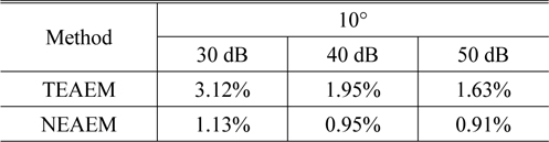
The results of accuracy analysis using the TEAEM and NEAEM in the simulation experiment
[TABLE 2.] The results of stability analysis using the TEAEM and NEAEM in the simulation experiment

The results of stability analysis using the TEAEM and NEAEM in the simulation experiment
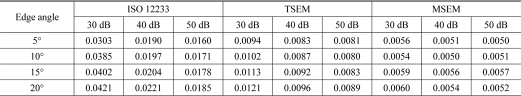
The accuracy of the MTF estimation based on the three different methods is analyzed by using images with edge angles of 5°, 10°, 15°, 20° and with SNRs of 30 dB, 40 dB, 50 dB. The results are shown in Table 3. The evaluation criterion is the root mean square error to the theoretic MTF curve, and the detailed calculation formula is defined as in Eq. (21):

The results of accuracy analysis using three MTF estimation methods in the simulation experiment
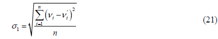
Where
Considering the results of the Table 3, the results of the ISO 12233 show that this method has a low accuracy, and when the noise is enhanced, the accuracy becomes lower, which shows that this method is easily affected by noise. With the edge angle becoming bigger, the marginal sections of the discrete ESF are sparse, which will amplify the influence of noise on differentiation calculation to obtain the LSF. As such, the ISO 12233 method is easily affected by noise and edge angle. The TSEM is more accurate than the ISO 12233 method. However, with the edge angle becoming bigger, the marginal sections of the discrete ESF are sparse, which will affect the precision of ESF fitting by using Fermi function. The MSEM is more accurate than the ISO 12233 method and the TSEM, and almost unaffected by varying noise and edge angle.
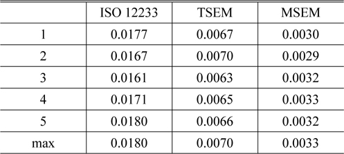
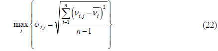
The stability analysis of the MTF estimation also uses five images with the same edge angle of 10° and with the same SNR of 40 dB. For every MTF estimation method, the referential MTF curve is the average MTF curve of the five measured MTF curves. The evaluation criterion is defined as the maximum of the root mean square error to the average MTF curve among the five measured MTF curves of every method. The detailed calculation formula is defined as in Eq. (22) and the results are shown in Table 4.

The results of stability analysis using three MTF estimation methods in the simulation experiment

Where
The results of Table 4 show that the MSEM is more stable than the ISO 12233 method and the TSEM. Therefore, the simulation experiment prove that the statistical calculation in extracting the edge angle and the ESF estimated based on the transfer function model make the MSEM more accurate and stable than ISO 12233 method and TSEM.
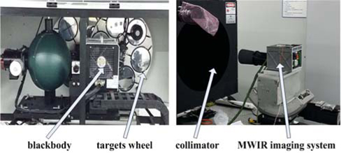
In order to test the practicability of the MSEM, an application experiment is performed to estimate the MTF of an MWIR imaging system by using the MSEM, ISO 12233 and TSEM. The testing setup is composed of blackbody radiation source, target wheels, collimator and MWIR imaging system, as shown in Fig. 6. For the MWIR imaging system, the spectral band is 4.2 μm ~ 4.8 μm, f-number is 2, focal length is 110mm, the detector is refrigeration type with 320×256 array focal plane and pixel size is 30 μm × 30 μm.
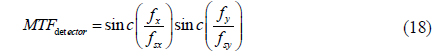
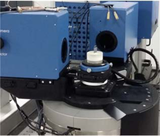
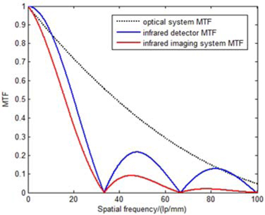
In the application experiment, to accurately evaluate these three methods, the referential MTF curve needs to be acquired first. Therefore, the curvature radius, thickness and material refractive index of every optical component are measured, and the intervals of optical components are also measured. Then the MTF curve of the optical system can be acquired by taking these measured values into the optical design software. The process of measuring material refractive index is shown in Fig. 7. The MTF curve of the infrared detector can be deduced from Eq. (18). As such, the product of the MTF curves of the optical system and the infrared detector is the MTF curve of the infrared imaging system, which is taken as the referential MTF curve, as shown in Fig. 8.
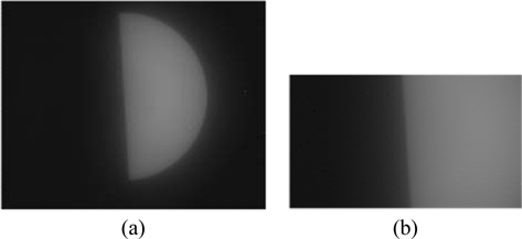
Using the knife edge target, the image of slant edge is acquired from the infrared imaging system, as shown in Fig. 9(a). A ROI for estimating the MTF is chosen on the image of slant edge, as shown in Fig. 9(b). For analyzing different methods, their ROIs are chosen identically in the image of slant edge to guarantee the validity of comparing the results. We rotate the knife edge target to generate some images with various edge angles. Then, these images are measured by using the MSEM, ISO 12233 and TSEM. The evaluation criterion is the root mean square error to the referential MTF curve from the zero to the Nyquist frequency, which is calculated by Eq. (21), and the results are shown in Table 5. The results of Table 5 show that the MSEM presents higher estimation accuracy and stability than the ISO 12233 and TSEM.
[TABLE 5.] The results of the MTF estimation in testing the MWIR imaging system

The results of the MTF estimation in testing the MWIR imaging system
In this paper, we propose an MSEM for MTF estimation of the optical imaging system. The MSEM is composed of a new edge angle extraction method and a new ESF fitting method. The kernel of the new edge angle extraction method is to use the gradient operator and a statistical calculation to estimate the edge angle. The ESF fitting method is built based on the transfer function model rather than using the approximate functions. A simulation experiment and an application experiment are performed to compare the MSEM with the TSEM and ISO 12233 method. With the edge angle and noise varying, the results of the experiments show that the MSEM is more accurate and stable than the TSEM and ISO 12233 method.