The binocular vision system was proposed in the 1870s, with the advantage of non-contact inspection and high measurement precision [1-3]. It provides flourishing developments in motion parameters testing, measurement of machine parts, parameter detection of micro-operating systems, 3D profile reconstruction [4-7], etc. It also gradually permeates into the aerospace, robot navigation, industrial measurement and bio-medical areas [8-13]. System calibration is the basis for binocular vision to obtain 3D coordinates. It provides the conversion relationship between the 2D coordinates of the images of the cameras and the 3D coordinates of the objects [3, 14, 15]. As the measurement accuracy of the binocular vision system depends on the camera calibration, the research on the camera calibration method has much theoretical importance and practical value.

Monocular vision measurement refers to the method of a camera taking a single photo for the measurement work [16]. It is difficult to achieve real-time large-scale mapping with a monocular camera, due to the purely projective nature of the sensor [17, 18]. Furthermore, the binocular vision system adopts two cameras, which obtain the 3D coordinates by means of matching the corresponding points [19-21]. In this paper, we study the global calibration method of the binocular vision systems that are located on different positions. The previous calibration method can be divided into three aspects by the dimension of the calibration object. The calibration objects of the binocular vision system include 1D objects, 2D objects and 3D objects [7, 22]. The 1D-object-based calibration was proposed a few years ago, which required an object consisting of more than three feature points [23]. The 1D calibration object can be conveniently moved, which is able to solve the block problems among multiple cameras. However, as the constraints provided by the unrestricted 1D object cannot completely identify the internal and external parameters of the camera, the motion of the 1D object is usually strictly constrained [24]. As for the method of the 2D calibration object, the calibration plate using a 2D gray-modulated sinusoidal fringe pattern is chosen to extract the phase feature points as the 2D calibration data [25-27]. The knowledge of the plane motion is not necessary in this calibration and the setup is easier. However, it cannot deal with the occlusion and depth-related problems [28, 29]. A 2D calibration object was reported to calibrate a binocular vision system used for vision measurement [12]. A precise calibration method was proposed for a binocular vision system which is devoted to minimizing the metric distance error between the reconstructed point and the real point in a 3D measurement coordinate system. The measurement accuracy of one binocular vision system is improved compared with the traditional method. For a vision measurement with multiple binocular vision systems, the measurement world coordinates of a binocular vision system are different from the ones of another binocular vision system considering the different positions of the 2D object. Therefore, the measurement world coordinates of a binocular vision system should be transformed to the ones of another binocular vision system. And then the front view of a 2D object is also difficult to simultaneously observe by multiple binocular vision systems. As for the 3D calibration object, the calibration object usually consists of two or three planes orthogonal to each other [30, 31]. The highest accuracy is usually obtained by using a 3D calibration object [32]. But this approach requires expensive calibration apparatus and an elaborate setup [20, 33]. A global calibration method of a laser plane is proposed, adopting a 3D calibration board to generate two horizontal coordinates and a height gauge to generate the height coordinate of the point in the laser plane [34]. The method is performed by a camera and a 3D calibration object. However, a 3D object is unable to calibrate the measurement system that consists of multiple binocular vision systems. A binocular vision system captures the images of the front view of the 3D object while the binocular vision system opposite to the former system is blocked by the back view of the 3D object. The blocking problem in the 3D calibration makes the simultaneous observation by all involved cameras impossible. Thus, we propose a three-degrees-of-freedom (three-DOF) calibration method that translates the 3D calibration board and rotates it to solve the view block problems between opposite binocular systems. The measurement coordinates of multiple binocular vision systems are also unified in a unique coordinate system.

A three-DOF global calibration method for binocular vision measurement is explored in this paper, which unites the measurements of the binocular vision systems at different positions into a single world coordinate system. The rest of this paper is organized as follows: Section 2 presents the principle of the three-DOF global calibration system that calibrates the binocular systems at the original, coaxial and diagonal positions. Section 3 proposes a three-DOF calibration model. According to the model, the coordinates of the feature points at the coaxial and diagonal positions are unified into a same world coordinate system. Section 4 outlines the global calibration experiments in coaxial and diagonal positions. Section 5 summarizes this paper.

The 3D calibration board is chosen as the benchmark of a single measurement system with binocular vision, which takes advantage of the simple and accurate calibration process. However, it is difficult to perform the global calibration among several binocular measurement systems in a large view field because of the limited size of the 3D calibration board and the perspective blocking problem.

Considering the complicated process to manufacture a large 3D calibration board, we present a three-DOF calibration system that makes the 3D calibration board move along the precise rail with a known distance and rotate around the turntable with an angle in the large view field. The three-DOF global calibration system unites the measurement results of the binocular vision systems at different positions into a single world coordinate system.

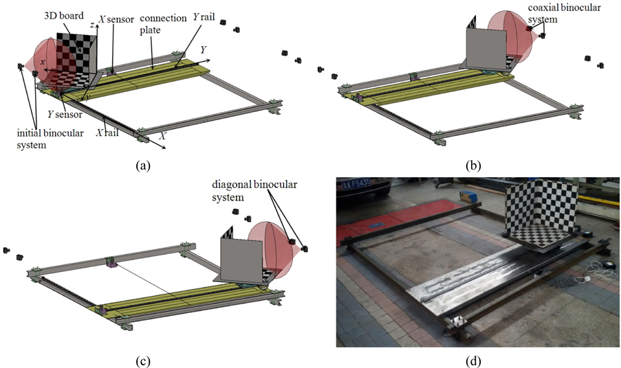
The structure of the global calibration system for binocular measurement systems is shown in Fig. 1. The three-DOF calibration system is mainly composed of a translational subassembly and a rotational subassembly. The translational subassembly mainly consists of a base frame, a connection plate, an X direction rail, an X direction displacement sensor, a Y direction rail and a Y direction displacement sensor, etc. The rotational subassembly is mainly composed of a 3D calibration board, a turntable, etc. The global calibration objects are the binocular measurement systems at the coaxial and diagonal positions. Three groups of the binocular systems are placed at the initial, coaxial and diagonal positions, respectively. Figures 1(a) and 1(b) show the calibration process of two groups of the binocular systems at the initial and coaxial positions. In the calibration, only one group of binocular system captures the images of the positive side of the 3D calibration board. Therefore, the rails and the turntable are utilized to move the 3D calibration board along the Y direction rail and rotate around from the initial position to the coaxial position on the other side. The binocular system at the coaxial position captures the images of the positive side of the 3D calibration board after translating and rotating 180 degrees. Figure 1(c) shows the calibration process of the binocular system in the diagonal position. In the calibration, the 3D calibration board still has to move along the X direction rail to the diagonal position. Then the binocular system in the diagonal position captures the images of the positive side of the 3D calibration board. The translation displacements and the rotation angle are measured by the X, Y direction sensors and the turntable, respectively. The measurement results of the binocular systems at different positions are ultimately unified into the world coordinate system. The world coordinate system is determined by the initial position of the calibration board.

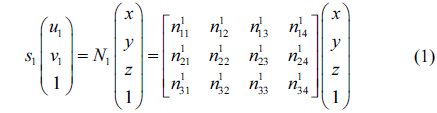
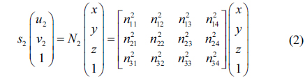
The imaging model of the binocular vision is indicated as [4]

where (x, y, z) is the 3D coordinate of a spatial point P, (u₁, v₁), (u₂, v₂) respectively represent the 2D coordinates of the corresponding points in the images captured by the two cameras, s₁, s₂ are non-zero scale factors, N₁, N₂ are the projection matrices of the two cameras. The projection matrix of the camera imaging model is calibrated by the relationship between 3D world coordinates and 2D image coordinates.

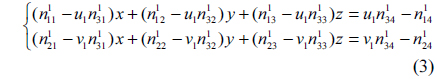
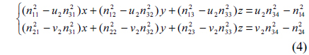
By eliminating the two scale factors s₁ and s₂ in Eqs. (1) and (2), the equations are described as

From Eqs. (3) and (4), the 3D coordinates of the feature points are reconstructed by the transformation matrices and image coordinates of the feature points.

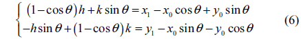
When we globally calibrate the binocular system on the coaxial or diagonal position, the 3D calibration board is moved from the initial position to the coaxial or diagonal position of the rectangle constructed by the frames. A laser projector is adopted to project a global horizontal laser plane at the initial position. Two horizontal lines on the calibration plate coincide with the laser plane by adjusting the height of the calibration board. Thus, the z direction values of the feature points are invariable when the calibration board moves to different positions. Therefore, the global calibration model is simplified from 3D to 2D.

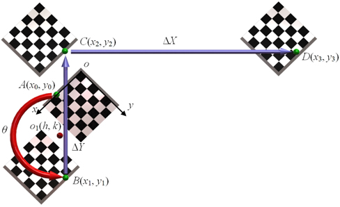
The intersection point of the three planes of the 3D calibration board in the initial position is taken as the global origin o of the world coordinate system o-xy. Then two images of the 3D calibration board are collected by the binocular system in the initial position. The 2D coordinates of the feature points are extracted from the two images. The 3D world coordinates are obtained from the size of the small square on the calibration board. The 2D image coordinates and the 3D world coordinates of the feature points in the initial position are known values, therefore, the transformation matrices are calibrated by Eqs. (3) and (4). Then the 3D world coordinates are reconstructed by the 2D image coordinates and the transformation matrices.

Three-DOF calibration model is shown in Fig. 2. When the binocular system on the coaxial position is globally calibrated, the 3D calibration board on the initial position rotates around the axis of the turntable, moves along the Y direction rail and finally arrives in the view field of the binocular system on the coaxial position. When we globally calibrate the binocular system on the diagonal position, the 3D calibration board on the coaxial position should move along the X direction rail and finally arrive in the view field of the binocular system on the diagonal position.

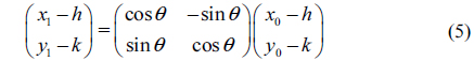
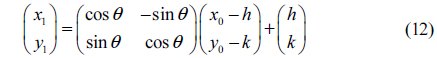
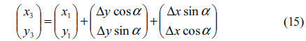
The feature points of the 3D calibration board are purely rotated around the axis of the turntable, while the feature points in the rotation formula should be rotated around the origin of the coordinate system. Therefore, the misalignment between the axis of the turntable and the origin of the coordinate system should be considered when we perform the rotation transformations of the feature points. The o-xy world coordinate system is determined by the initial position of the 3D calibration board. Let o₁ be the projection point of the rotation axis of the 3D calibration board in the o-xy coordinate system. The coordinate of o₁ is (h, k) in the o-xy coordinate system. The coordinate of the feature point A is (x₀, y₀) in the o-xy coordinate system. First, as the feature points are rotated around the o₁z₁ rotation axis, the o-xy coordinate system is moved to the o₁-x₁y₁ coordinate system. The coordinate of the feature point A is (x₀-h, y₀-k) in the o₁-x₁y₁ coordinate system. Then the 3D calibration board is rotated around the o₁z₁ axis with a small angle θ. The value of the angle θ is obtained from the scale on the hand wheel of the turntable. After the rotation of the angle θ, the feature point A is moved to the point B. The coordinate of the point B is (x₁, y₁) in the o-xy world coordinate system. Thus the coordinate of the point B is (x₁-h, y₁-k) in the o₁-x₁y₁ coordinate system. According to the formula of the rotation matrices, the relationship between the point A and B in the o₁-x₁y₁ coordinate system is given by

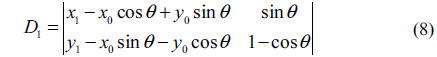
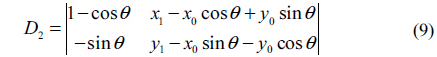
The result of the above matrix multiplication is represented as

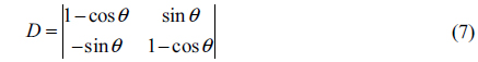
The coefficient determinants are represented by

The coordinates (x₀, y₀) and (x₁, y₁) of the point A, B in the o-xy world coordinate system are reconstructed by Eqs. (3), (4). So the coefficient determinants D, D₁, D₂ are calculated by the coordinates of the point A and B. According to Cramer’s rule, h and k are given by

Therefore, the 3D calibration board is rotated by a known angle θ to get the coordinate (h, k) of the projection point o₁. After calibrating the coordinate (h, k) of the point o₁, the coordinate (x₁, y₁) of the point B in the o-xy world coordinate system is obtained by the coordinate translation and rotation with a known arbitrary θ angle. According to Eq. (5), the coordinate (x₁, y₁) of the point B in the o-xy world coordinate system is given by

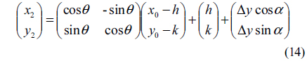
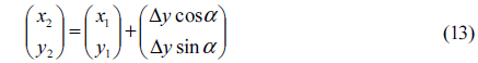
In the calibration of the binocular system at the coaxial position, the 3D calibration board is rotated by 180 degrees and moved along the Y direction to the coaxial position within the view field of the cameras. The point B moves along the Y direction with a distance of ΔY to the point C. The coordinate of the point C is (x₂, y₂) in the o-xy world coordinate system. As the ΔY direction is not parallel with the y direction, the relationship between the point C (x₂, y₂) and the point B (x₁, y₁) is represented by

where α is the angle between the ox axis of the world coordinate system and the Y direction rail.

As the point C and the point A are respectively obtained by the binocular system at the coaxial position and the initial position, substituting Eq. (12) into Eq. (13), the relationship between the point C (x₂, y₂) and the point A (x₀, y₀) is given by

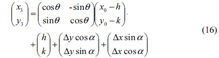
In the calibration of the binocular system at the diagonal position, the 3D calibration board is rotated by 180 degrees and moved along the Y direction and X direction to the diagonal position within the view field of the cameras. In other words, the 3D calibration board needs to be moved along the X direction on the basis of the coaxial position. The point C moves along the X direction with a distance ΔX to the point D. The coordinate of the point D is (x₃, y₃) in the o-xy world coordinate system. The relationship between the point D (x₃, y₃) and the point B (x₁, y₁) is represented by

As the point D is obtained by the binocular system at the diagonal position, substituting Eq. (12) into Eq. (15), the relationship between the point D (x₃, y₃) and the point A (x₀, y₀) is

The coordinate (x₀, y₀) of the feature point on the 3D calibration board can be determined by the location of the corner point on the checkerboard. The coordinate (h, k) of the projection point of the rotation axis is obtained by Eqs. (10), (11). The values of ΔX and ΔY are shown by the displacement sensors that are installed on the two directions of the three-DOF calibration system. The rotation angle θ and angle α are read from the scale on the hand wheel of the turntable. In conclusion, the feature point C is captured by the binocular system at the coaxial position. The coordinate (x₂, y₂) of the point C in the world coordinate system is obtained from Eq. (14). The feature point D is captured by the binocular system on the diagonal position. The coordinate (x₃, y₃) of the point D in the world coordinate system is obtained from Eq. (16).

In the experiments, the size of the selected 3D calibration board is 500 mm × 500 mm × 500 mm. The plane pattern of the calibration board is a square checkerboard with the same size of 60 mm × 60 mm. The evenly distributed 18 points in the two sides of the calibration board are taken as the feature points. The measurement scope and accuracy of the displacement sensors in the X direction and the Y direction are 2000 mm and 0.05%, respectively. The turntable is the equipment to measure the rotation angle of the 3D calibration board. The accuracy of the turntable is ±40″. The laser level is the device to level the three-DOF global calibration system. The horizontal accuracy of the laser level is ±1 mm.

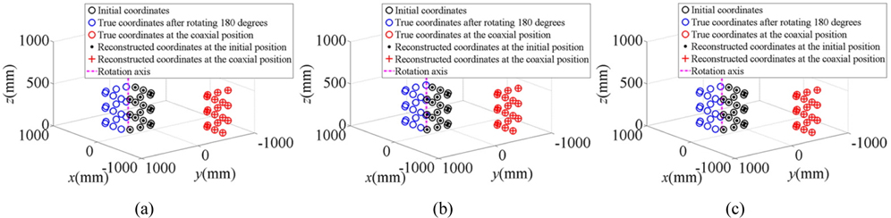
Three global calibration experiments are conducted to unite the measurement results of the binocular vision system at the coaxial position into the world coordinate system at the initial position. The 3D calibration board moves along the Y direction after rotating 180 degrees. The coaxial distances along the Y direction are 1428 mm, 1296 mm and 1358 mm in the three experiments. When the calibration is performed, the 3D calibration board is put at the position of the initial world coordinate system. The world coordinates of the 18 feature points are calculated by the size of the checkerboard. Then the transition matrices of the two cameras are calibrated based on the world coordinates of the feature points and the image coordinates of the 3D calibration board captured by the binocular system at the initial position. Furthermore, the 3D calibration board is rotated by a known angle. As the projection point o₁ is the rotation axis projected in the horizontal plane, the coordinate (h, k) of the projection point o₁ is obtained from Eqs. (10), (11). The known angle in the test is 4 degrees. The coordinates of the rotation axis in the three experiments are (258.118, 251.362), (277.352, 212.805) and (257.953, 245.333), respectively. Finally, the 3D calibration board is rotated by 180 degrees and moved to the place in front of the binocular system at the coaxial position. The angle α between the ox axis and the Y direction of the 3D calibration board is 45 degrees. The 3D calibration board is rotated and moved to the coaxial position. The world coordinate of the feature point (x₂, y₂) is obtained from Eq. (14).

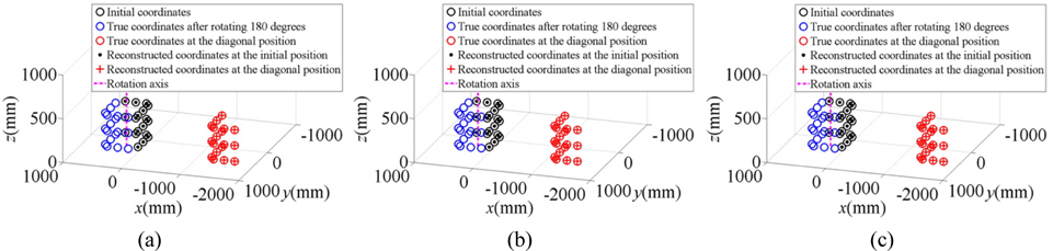
According to the calibration processes of the coaxial position, the 3D world coordinates at different positions are reconstructed in Fig. 3. In the experiments, we make a comparison between the world coordinates of the reconstructed feature points and the true feature points. The coordinates of the reconstructed feature points are obtained from the image captured by the binocular system. In Fig. 3, the reconstructed feature points on the 3D calibration board are rotated by 180 degrees from the initial position. Then the board moves along the coaxial direction and finally reaches the coaxial position. The reconstructed and the true coordinates of the feature points at the coaxial position are in coincidence.

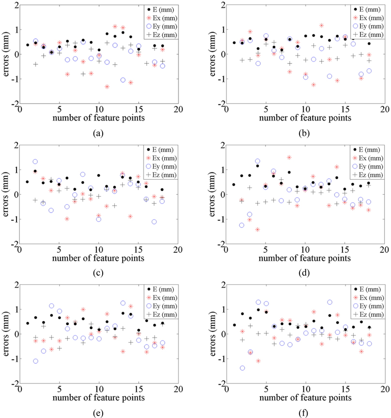
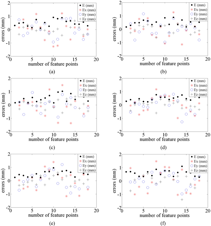
In order to further analyze the accuracy of the reconstructed results, in the three experiments, the differences between the true and reconstructed 3D coordinates of the feature points at the initial position are indicated in Figs. 4(a)~4(c), respectively. The differences between the true and reconstructed 3D coordinates of the feature points at the coaxial position are indicated in Figs. 4(d)~4(f), respectively. E_x, E_y, E_z are the differences between the true and reconstructed 3D coordinates of the feature points at the x, y and z direction, respectively. E is the root-mean-square of the errors of the feature points.

In Figs. 4(a)~4(c), the scope of the maximal errors about the 3D calibration board at the initial position is −1.5 mm−1.5 mm in the three experiments. The root-mean-square errors of the first group are 0.725 mm, 0.461 mm and 0.348 mm in the x, y and z directions, respectively. The total root-mean-square error of the group is 0.535 mm. The root-mean-square errors of the second group are 0.733 mm, 0.581 mm and 0.261 mm in the x, y and z directions, respectively. The total root-mean-square error of the group is 0.561 mm. The root-mean-square errors of the third group are 0.574 mm, 0.646 mm and 0.311 mm in the x, y and z directions, respectively. The total root-mean-square error of the group is 0.530 mm. In Figs. 4(d)~4(f), the scope of the maximal errors about the 3D calibration board at the coaxial position is also −1.5 mm−1.5 mm in the three experiments. The root-mean-square errors of the first group are 0.732 mm, 0.607 mm and 0.282 mm in the x, y and z directions, respectively. The total root-mean-square error of the group is 0.573 mm. The root-mean-square errors of the second group are 0.563 mm, 0.642 mm and 0.289 mm in the x, y and z directions, respectively. The total root-mean-square error of the group is 0.520 mm. The root-mean-square errors of the third group are 0.561 mm, 0.687 mm and 0.222 mm in the x, y and z directions, respectively. The total root-mean-square error of the group is 0.528 mm. In conclusion, the scope of the reconstructed errors after the rotation and movement of the 3D calibration board is the same as the scope of the reconstructed error at the initial position.

In Fig. 4(a), the errors’ scope is −1.5 mm-1.5 mm in the x direction. The errors’ scope is −1.5 mm−1 mm in the y direction. The errors of the feature points are in a dispersal distribution in the y direction. The errors mainly distribute in the scope of −0.5 mm−0.5 mm in the z direction. In Fig. 4(d), the errors dispersedly distribute in the scopes of −1 mm−1 mm and −1.5 mm−1.5 mm in the x and y directions, respectively. However, the errors in the z direction mainly distribute in −0.5 mm−0.5 mm. In Figs. 4(b)~4(f), the scopes of the errors in the x and y directions are both −1.5 mm−1.5 mm. The errors in the z direction mainly distribute in the scope of −0.5 mm−0.5 mm. Therefore, the errors in the z direction are less than the errors in the x and y directions. The direction with the minimal reconstructed errors is the perpendicular direction to the baseline and the measurement distance.

Three global calibration experiments are performed to unite the measurement results of the binocular vision system at the diagonal position into the world coordinate system at the initial position. The 3D calibration board moves along the Y direction and X direction after rotating a small angle. The distances along the Y direction are 1121 mm, 1262 mm and 1289 mm in the three experiments. The distances along the X direction are 1271 mm, 1339 mm and 1381 mm in the three experiments. The coordinates of the rotation axis in the three experiments are (260.467, 243.225), (270.628, 253.230) and (253.413, 243.256), respectively. Finally, the 3D calibration board is rotated by 180 degrees and moved to the place in front of the binocular system at the diagonal position. The world coordinate of the feature point (x₃, y₃) is obtained from Eq. (16).

According to the calibration processes of the diagonal position, the 3D world coordinates at different positions are reconstructed in Fig. 5. In Fig. 5, the reconstructed feature points on the 3D calibration board are rotated by 180 degrees from the initial position. Then the board moves along the Y direction, X direction and finally reaches the diagonal position. The true and reconstructed the coordinates of the feature points at the diagonal position are basically in coincidence.

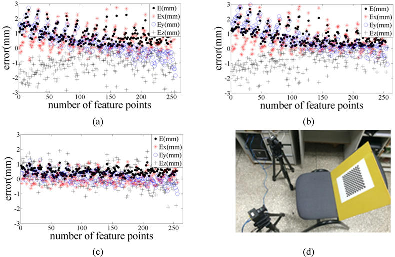
In the three experiments, the differences between the true and reconstructed 3D coordinates of the feature points at the initial position are indicated in Figs. 6(a)~6(c), respectively. The scope of the maximal errors about the 3D calibration board at the initial position is −1.5 mm−1.5 mm. The root-mean-square errors of the first experiment are 0.690 mm, 0.571 mm and 0.312 mm in the x, y and z directions, respectively. The total root-mean-square error of the group is 0.548 mm. The root-mean-square errors of the second experiment are 0.629 mm, 0.550 mm and 0.301 mm in the x, y and z directions, respectively. The total root-mean-square error of the group is 0.513 mm. The root-mean-square errors of the third experiment are 0.757 mm, 0.528 mm and 0.321 mm in the x, y and z directions, respectively. The total root-mean-square error of the group is 0.564 mm. The differences between the true and reconstructed 3D coordinates of the feature points at the diagonal position are indicated in Figs. 6(d)~6(f), respectively. In the three experiments, the scope of the maximal errors about the 3D calibration board at the diagonal position is also −1.5 mm−1.5 mm. The root-mean-square errors of the first group are 0.572 mm, 0.571 mm and 0.284 mm in the x, y and z directions, respectively. The total root-mean-square error of the group is 0.495 mm. The root-mean-square errors of the second group are 0.696 mm, 0.604 mm and 0.283 mm in the x, y and z directions, respectively. The total root-mean-square error of the group is 0.556 mm. The root-mean-square errors of the third group are 0.819 mm, 0.489 mm and 0.318 mm in the x, y and z directions, respectively. The total root-mean-square error of the group is 0.627 mm. In conclusion, the scope of the reconstructed errors after the rotation and movement of the 3D calibration board is the same as the scope of the reconstructed error at the initial position.

In Fig. 6(a), the scopes of the errors in the x direction and y direction are −1.5 mm−1.5 mm, −1.5 mm−1 mm, respectively. The errors in the z direction mainly distribute in −0.5 mm−0.5 mm. In Fig. 6(d), the scopes of the errors in the x direction and y direction are −1 mm−1 mm, −1.5 mm−1.5 mm, respectively. The errors of the x and y directions are in a dispersal distribution. However, the errors in the z direction mainly distribute in the scope of −0.5 mm−0.5 mm. In Figs. 6(b)~6(f), the scopes of the errors in the x and y direction are both −1.5 mm−1.5 mm. The errors in the z direction mainly distribute in −0.5 mm−0.5 mm. Therefore, the minimal reconstructed errors also distribute in the direction that is perpendicular to the baseline and the measurement distance.

We perform calibration experiments for a binocular vision system with a 2D calibration board. The projection matrices of two cameras are determined by Zhang’s method [27]. The experimental results are shown in Figs. 7(a)~7(d). The measurement results are also evaluated by reconstructed errors. The experimental root-mean-square errors between the true and reconstructed 3D coordinates of the feature points are 0.989 mm, 1.048 mm and 0.546 mm The root-mean-square errors of the three group experiments are 0.963 mm, 0.952 mm, 0.421 mm in the x direction, 0.989 mm, 0.850 mm, 0.378 mm in the y direction and 1.014 mm, 1.292 mm, 0.758 mm in the z direction. The measurement accuracy of the three-DOF calibration method is close to the measurement accuracy of the 2D calibration method. The view block problem of multiple binocular systems is also solved by the three-DOF calibration method.

This paper addresses a global calibration method with a three-DOF calibration system. The model of the three-DOF global calibration system is studied in this paper. The 3D calibration board is moved to an arbitrary position in the model. According to the motion law of the three-DOF global calibration system at different positions, we deduce the global calibration model of the binocular systems at different positions. The measurement results of the binocular systems at different position are unified into a world coordinate system that is determined by the initial position of the calibration board. Three experiments of the binocular systems at the coaxial and diagonal positions are respectively conducted to verify the global calibration method of the vision measurement systems. The root-mean-square errors between the true and reconstructed 3D coordinates of the feature points are 0.573 mm, 0.520 mm and 0.528 mm at the coaxial position, respectively. The root-mean-square errors between the true and reconstructed 3D coordinates of the feature points are 0.495 mm, 0.556 mm and 0.627 mm at the diagonal position, respectively. The reconstructed errors of the global calibration system for the binocular measurement systems are minimal at the direction that is perpendicular to the baseline and the measurement distance. The method unities the measurement results of the binocular vision systems at different positions into the same world coordinate system, which is of great significance in the research field of the vision-based measurement.