There is no doubt that adaptive optics (AO) is the most promising method to compensate wavefront disturbance in free space optics communication (FSO). In order to improve the performance of the AO system described by discrete-time linear system model with time-delay and implicit phase turbulent model, new controllers based on a Kalman filter and its extensions are proposed. Based on the standard Kalman filter, we propose a fading memory filter to deal with the ruleless strong interference; sequential and U-D filters are applied to reduce implementation complexity for the embedded controllers. Theoretical analysis and the numerical simulations show that the proposed fading memory filter can upgrade the performance for AO systems in consideration of the unforeseen strong pulse interference, and the sequential and U-D filters perform well compared with a Kalman filter.
The free space optical (FSO) communication system is widely used in the telecommunication community for both space and ground wireless link and last-mile applications due to its unregulated spectrum, large bandwidth potential, relative low power requirement, low bit error rate (BER) and ease of redeployment. However, atmospheric turbulence in this system will bring phase disturbances along propagation paths that result in intensity fluctuation (scintillation), beam wandering and beam broadening at the receiver leading to significant decrease of coupling efficiency at the receiving terminal, which influences the stability and reliability of the FSO communication systems. Adaptive optics (AO) systems are used to compensate time-varying wavefront distortions by using noise and measurement delay [1]. The objective of AO system in astronomy or satellite-to-ground free space laser communication is to minimize the effects of atmospheric aberrations of received signals [2, 3]. A feedback loop is the core of an AO system: namely the incoming uncorrected wavefront is reflected from a deformable mirror (DM), the reflected wavefront is measured by a wavefront sensor (WFS), and the shape of the DM is adjusted based on the measurements of the WFS to correct the wavefront distortions [4]. The performance of AO system can be significantly affected by the control algorithm used in the system. Therefore, control and performance optimization of AO could be one of the key research issues.
Most controllers normally reconstruct the WFS measurements first. Modal bases using Zernike [5], Karhunen-Loeve function [6], and system modes are used by modal controllers [4]. The reconstructed error wavefront serves as the input of the compensation algorithm. The Linear-quadratic-Gaussian (LQG) control formulation can be used in AO systems to design the controller that minimizes the error wavefront variance in lots of studies referring to this issue. Different linear AO systems and turbulence models, primarily the auto-regressive model, are studied for the performance analysis of a complete AO telescope using the LQG controller [7]. The controller generates optimal inputs for the DM by giving the wavefront sensor measurements, the statistical characteristics of these measurements and noise. An interesting LQG design technique is used in an AO system by modeling the first 14 Zernike modes (ignoring piston mode) with spectra generated by first-order independent Markov models in [8]. In [9], the proposed controller, which uses state-feedback of wavefront estimate obtained from Kalman filter, incorporates a model of the atmospheric wavefront by a second-order auto-regressive model.
Controller using Kalman filter and state feedback in discrete-time AO-loop model has been proposed by some studies. Several excellent works addressing the control of a linear AO system are provided in [4, 10-15]. A diagonal modal controller based on an LQG modal of the modes and the measured modal spectra are given in [10]. In this controller design, the problem of the minimum variance AO controller as an LQG problem [4] is formulated. Then under a discrete-time model considering the temporal dynamics of the DM and the atmospheric aberration, the computational loop delay and the frame integration of WFS are obtained. Later, a method to compute the average variance of the residual of an AO system is developed [11]. As a useful complement, the extension of a discrete time model of an AO system is also given, in which the WFS produces measurements at discrete-time intervals by integrating the input wavefront over a part of frame [12]. The hybrid LQG controller is presented in [13] from the equivalent discrete-time model in [11]. The solution is given by two discrete-time algebra Riccati equations (AREs). Furthermore, this work is extended by the analysis of a model with input delay [14] occurring immediately after zero-order holder (ZOH). The model presents the same performance as the model presented in [11, 13], since there is no requirement for the delayed IWF, the order of the input-delay model is low and the IWF model does not represent the loop delay. In consequence, the resulting order of the optimal controllers based on the input-delay model can be reduced without relying on model reduction techniques to have clear model structure. An independent study in [15] provides a finite dimensional state variable model for the systems with CCD-based measurements.
In addition, serious works on the data-driven H2 optimal control are also proposed [16-19]. It is well understood that H2 control also belongs to the LQG control because of the same optimization object. The estimation of the key parameters of the multi-variable state-space model of the wavefront disturbance is provided in [16] by providing a full description of the spatio-temporal statistics by open-loop wavefront slope data. A control law without AREs is proposed in [17], it is on the assumption that the only dynamics in the system is a unit-sample delay between measurement and correction. Based on these works, [18] and [19] present a data-driven H2-optimal control design strategy by taking the pseudo-inverse of the WFS matrix fully depending on measured data. Their disturbance model is reasonable only if the statistical properties of the wavefront change on a time scale that is long with respect to that of the fluctuations.
Based on the above discussion and analysis, the model construction of the discrete-time AO system and the application of the LQG control to this model in different aspects are very significant contributions. However, in our study, we focus on the various Kalman filters in an AO system with the models more conveniently given in [1, 20-24]. A closed-loop control law resulting from a global optimization is proposed in [20] to demonstrate the efficiency in the context of multi-conjugate adaptive optics (MCAO). This law is based on the assumption that the DMs are fast enough compared with sampling period, which is often valid in astronomical applications. The work presents an explicit frame that we can combine the linear quadratic (LQ) control (state feedback) with Kalman filter to predict or estimate the turbulence in the next frame by solving an optimization problem.
Under the same frame, the issue of residual phase variance minimization in AO loops from control perspective is addressed in [1]. This study indicates that a suitably modeled AO system can be divided into an optimal deterministic control problem and an optimal estimation problem. The solution of this problem is a linear quadratic (LG) control with a Kalman filter. Actually, a convenient framework for the analysis of AO controllers is provided in [1] with an implicit phase turbulence model. Based on the framework, some interesting experimental studies are also given in [21-24], for example, vibrations, windshake, and tracking are considered in [21, 22, 24] which illustrate the experimental validation of the control law that LQG can provide an optimal correction of the vibrations in the case of residual phase minimal variance. The method with experimental proof in [23] is fundamentally the same as that in [1]. In addition, basically by following Caroline Kulcsár’s model [1], an improvement for bad performance of Kalman gain from some unrealistic assumptions is presented in [25]. Moreover, the problem of efficient computation and implementation of a Kalman filter to predict frozen flow turbulence with von Kármár spatial correlation is addressed in [26]. However, this study is limited by the assumption of the wavefront phase propagations in time as a wave with a constant velocity (Taylor frozen flow assumption). A state-space disturbance model and associated prediction filter for aero-optical wavefront are given in [27-29]. This model can be obtained by subspace system identification method proposed in [30] from a sequence of measured wavefronts using the Karhunen-Loéve modes in [28]. With the basic idea, the advantage of less real-time computation of the optimal LTI controller compared to the adaptive controller in [31, 32] is discussed in [27]. The results from a real-time implementation of an optimal controller on the PALM-3000 adaptive optics system are given. However, the un-modeled dynamics still affect control performance and robustness, which is the problem for further study. Earlier studies do not refer to a Kalman filter even they can also be classified in the filter based controller in [31-35].
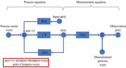
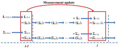
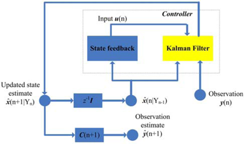
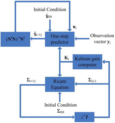
The effective framework in [1, 20-24] is based on a linear description of constitutive elements of an AO loop through the combination of Kalman filter and LQ (state feedback) to produce input signals for DM. This paper extends Caroline Kulcsár’s works and presents the performance of Kalman filter and its variants in classic discrete-time linear AO systems. To give a brief and clear description, our basic idea is given in Fig. 1 and Figure 2. We temporally ignore the real meaning of every signal here and its detailed explanation will be presented in Section 2.
Figure 1 shows a standard state space description of discrete-time linear system. The task is to obtain best
FSO system requires highly accurate structure and necessary implementation consideration to the real-time system. When the Kalman filter is used on a real FSO system it may not work well, even though the theoretical result is correct, since any system model errors, unforeseen pulse interference from electric sparks or strong electromagnetic wave or uncertainty may aggravate the performance. To deal with the un-normal conditions we should study how to design a suitable Kalman filter for the consequence of higher transmission rate requirement of the FSO system. Our object is to recover the qualified running condition from the possible un-normal ‘trap’ as soon as possible to ensure the stability and the communication performance. In addition, we need ‘self-healing’ property in the FSO system with high requirement for instantaneity. In this respect, we develop a fading memory filter to improve the performance of ‘self-healing’ by introducing a forgetting factor to put more importance for current measurement to quickly realize ‘self-healing’.
Another problem for Kalman filter is the application limitation in embedded controller, since it normally requires matrix inversion which is complicated for the calculation of the embedded controller. In this study we try to present two kinds of Kalman filter without relying on the matrix inversion calculation, sequential filter and U-D filter for discrete-time FSO-AO-loop, which could be implemented in an embedded system to counteract the dramatically changed circumstance.
This paper is organized as follows. We recall the linear discrete-time model of AO in Section 2 for addressing the residual phase variance minimization in discrete AO loops. Then the traditional controller under realistic assumptions is introduced in Section 3 with the performance discussion of different Kalman filters. A comparison is illustrated in Section 4 on the end-to-end AO bench simulators implemented by MATLAB to present the different characteristics of the filters. Finally, conclusions are presented in Section 5.
II. CLASSIC LINEAR SYSTEM MODELS AND KALMAN FILTER
This section presents a general review of the classic discrete-time model and state space model of AO since it is the central part of FSO. We use Caroline Kulcsár’s model [1, 20, 21, 23] in this study.
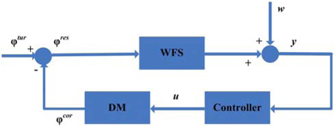
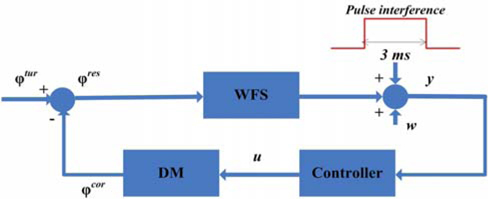
The classic configuration of a closed loop AO system is presented in Fig. 3 [1, 23]. The light comes from a guide star or a laser transmitter on the satellite. The correction phase φ cor is generated by the DM to compensate the turbulence phase φ tur, and
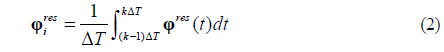
where the average value of residual phase res in one time interval Δ

where∥・∥represents the Euclidean norm. Here we assume all phases are expanded on the Zernike basis [5]. In addition, many researchers prefer to use the Strehl ratio (SR), namely the central peak of the point spread function (PSF) achieved by the receiver over the central peak of the PSF without the turbulence, and SR can be approximated by

where
On the assumption that both the delay in WFS measurement and the DM response is in one time interval Δ

where D is the WFS matrix and

where N is the influence metric of the DM.
Under the “full information” hypothesis that φ

where Nt is the transposition of N.
We can simply replace in Eq. (6) by which is the minimum-variance estimator of based on Γ

where .
2.2. State Space Model of Discrete-time Delay AO System
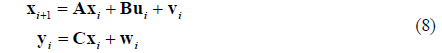
A state space linear time-invariant model is described in the following form

where A, B and C are matrices of appropriate dimensions, v
The state vector is then

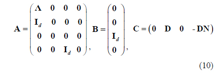
The choice for the state vector is not unique, and different state vectors may describe the same input-output behavior. The reason for choosing this state vector is explained in [1, 20]. The stochastic state space model is now completely defined by (8) as

where is used to present dynamic turbulence by a one-order auto-regressive model (interested readers can get a detailed description in [1, 8, 25, 36])

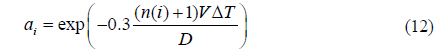
where is a Gaussian white process with covariance matrix , and is assumed to be a diagonal matrix with elements
where

where Σφ
Then the optimal control u directly obtained from (7) has the state feedback form

If we want to get optimal control u, we need Kalman filters to estimated space vector , such that the control will be realized. Note that the proposed methods are just for the stable temporal atmospheric conditions under which the wind speed and direction are nearly stationary. The Kalman filter based AO technology has its inherent characteristic that the prior knowledge of atmosphere turbulence has to be known. This corresponds to the more stationary communication environment of breeze or weak turbulence. In most earth satellite links, the wavefront distortions from atmospheric turbulence often occur in the near field of telescope aperture, and the intensity fluctuations or scintillations can be considered relatively weak and stationary within a period of time [1, 20, 40].
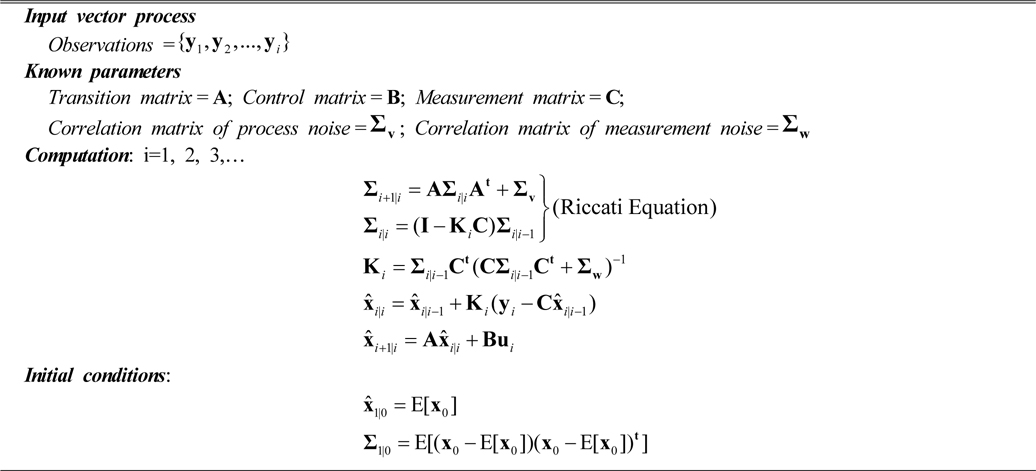
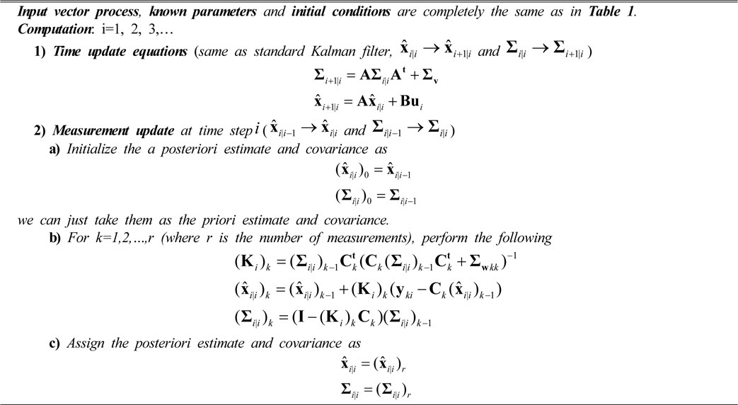
We only give the workflow of Kalman filter used in this paper (see Table 1 and Fig. 4) because it has been illustrated in some related works [1, 20-24].
[TABLE 1.] Summary of Kalman filter based on one-step prediction in AO loop

Summary of Kalman filter based on one-step prediction in AO loop
In Table 1, is the filtered value of x at time
III. KALMAN FILTER AND ITS VARIANTS IN AO SYSTEM
FSO system is a real-time system with high operating speed. Once some unforeseen interference happens, the qualified running will be interrupted and Kalman filter based controller needs the ‘self-healing’ to recover to the normal operation quickly otherwise some necessary information may be lost in the FSO system with very high transmission rate. It is difficult to solve this problem by remodeling and analysis because unforeseen interferences are difficult to present in the system model. In this section we bring a forgetting factor for the design of the Kalman filter with ‘self-healing’ ability.
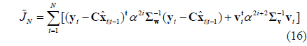
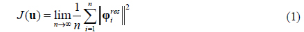
The designed Kalman filter estimates the sequence that minimizes the expectation of
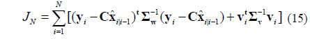
Instead of finding the filter that minimizes

where
In this regard, we need to define
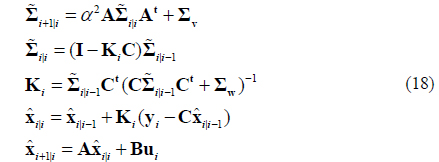
We can easily get the update equation from the standard Kalman filter

We see that the fading-memory filter is identical to the standard Kalman filter, with the exception that the time-update equation for the computation of the priori estimation-error covariance has
If
The analysis above is helpful to give a stable system when the unforeseen pulse interferences happen. Because the estimated value at this moment, which diverges from the normal estimation, is no longer to be trusted. In the next predictions, the modification makes the system discount the bad estimated value and give greater emphasis to the most recent measurements. By this way, the AO system can recover and converge to the qualified condition as soon as possible, which improves the ability of ‘self-healing’ and avoid the loss of information data. This causes the filter to be more responsive to measurements, which may result in the loss of optimality of the Kalman filter, but it may restore its performance on ‘self-healing’. It is better to have a theoretically suboptimal filter that works rather than a theoretically optimal filter that does not work. The greater responsiveness of the fading-memory filter to the current measurements makes the filter less sensitive to the modeling errors, and hence more stable.
Sequential Kalman filter is a great advantage, especially in an embedded system that may not have matrix routines (we are used to process matrices with MATLAB, unfortunately it is not that easy in an embedded system) to solve the problem of matrix inversion in practical applications.
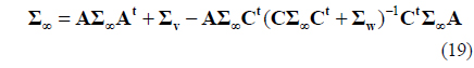
The studies about the “off-line” pre-operation to avoid the matrix routines [1, 20-24] make Σ

It may work under the condition of stationary global energy of the turbulence and the measured noise in the WFS. In other words, the system should work well in some adverse conditions where the environment changes producing significant disturbances of power (ΔΣv) and measured noise (ΔΣW) at some time spots. In this case, to keep better performance, AO controller must recalculate . It is clear that (19) is a nonlinear matrix equation, so that ΔΣ∞ is very hard to obtain. Thus the resultant steady-state optimal controller may work theoretically in particular experimental conditions but it should be treated with caution in practical applications. With this in mind, as a compromise, the Kalman-filter based controllers without matrix inversion are necessary and practical when the significant circumstance changes are detected.
To avoid matrix inversion, we implement the Kalman filter measurement-update equation by one measurement y

where C
[TABLE 2.] Sequential Kalman Filter in AO loop

Sequential Kalman Filter in AO loop
In Table 2, Σw
The sequential Kalman filter exactly counteracts the varying circumstance because the Kalman gain is not forced to be a steady constant. Once the environment changes, the proposed controller can dynamically update the Kalman gain without human interference.
The sequential Kalman filter requires r scalar divisions (where r is the number of measurements) in each time step. This is different from the standard Kalman filter depicted in Fig. 4.
U-D filtering is another method for easy implementation in the embedded systems. It is sometimes considered as a type of square root filtering. It increases computational cost of the filter but not as severely as the square root filter [38].
We need to decompose two
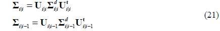
where and are
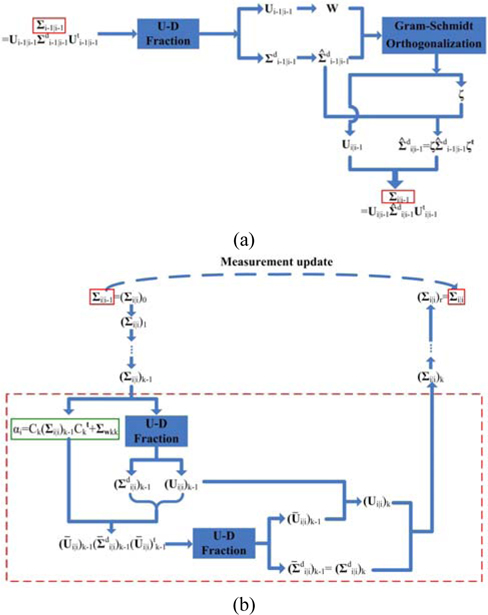
[TABLE 3.] U-D Kalman Filter in AO loop
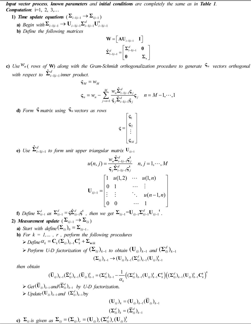
U-D Kalman Filter in AO loop
The U-D filter requires less computation than the general square root filter. At first sight, it may make us discouraged because of such a prolix and complicated description. Actually it is a simple iterative process without any matrix inversion; we can see Fig. 6 (a) and (b) to get deeper understanding.
The U-D filter can also avoid numerical difficulty, since solution of the Riccati equation should always be a symmetric positive semi-definite matrix theoretically, which is hard for computer or embedded system to guarantee because of the accuracy of the numerical calculation. Therefore, the U-D filter is a good algorithm to mathematically increase the estimate precision of the Kalman filter when high performance hardware is not necessary or available.
This experiment assumes that the AO system is a linear discrete-time loop, and the simulation parameters are taken from the works of Brice Le Roux [20] and Caroline Kulcsár [1]. Actually the object in this paper is to compare the performance of Kalman filters, so we would simplify the model only if the controllers are under the same preconditions. The beam diameter at transmitter is about a few centimeters, and the laser beam is adjusted to adapt to the deformable mirror diameter abstractly (~15 cm). We take the related parameters in (12) as
We approximate the DM influence function N by Gaussian Model as following
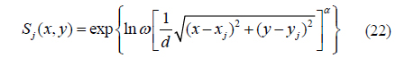
where 𝜔 is the coupling coefficient. (

where
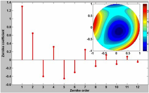
Figure 7 demonstrates an initial wavefront distortion Zernike coefficients of the introduced wavefront distortion and the static wavefront distortion on the top right corner. We obtain that the initial SR is 0.06 by numerical simulation of Phase Screen (PS), which implies more than 90% energy is lost in the propagation because of the atmosphere turbulence.
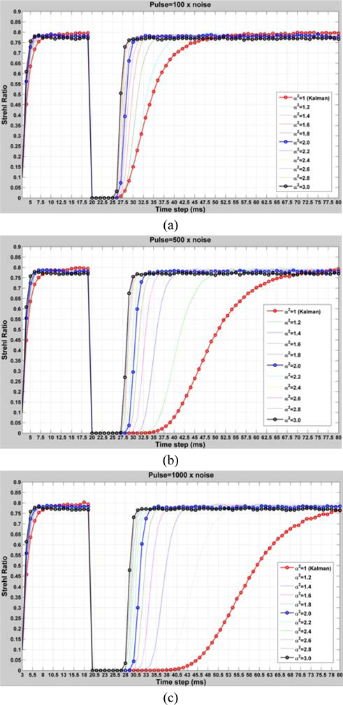
To illustrate the performance of the fading memory filter with ‘self-healing’, the simulated pulse interference is introduced into the WFS (as shown in Fig. 8) at the 20th time step. The pulse is very strong and assumed to last for a very short period, e.g. 0.003 s (3 time steps). The compensating results of the Kalman filter and the fading memory filter are shown in Fig. 9 (a), and the intensity of the pulse is assumed to be 100 times, (b) 500 times and (c) 1000 times larger than that of the measured noise w; The two filters can counteract the distorted wavefront, but the fading memory loses little optimality while providing the ‘self-healing’ ability when the pulse interference occurs.
When the pulse interference occurs at the 20th time step, SR sharply reduces. With the increasing pulse intensity from 100 w, 500 w to 1000 w, Kalman filter needs much more time to recover to the qualified operation (‘SR=0.75’ is defined as the qualified metric in this simulation, when SR >=0.75, it is considered as the ‘qualified operation’), precisely in 23 ms, 43ms and 55 ms respectively. When the fading-memory filter is adapted to FSO system, the time of ‘self-healing’ obviously reduces to less than 10ms. Therefore, the system performance is improved in the presence of the interference with fast response.
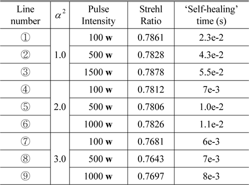
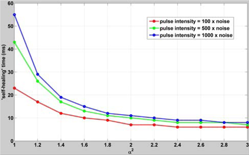
Figure 10 presents the consumed time for ‘self-healing’ from Fig. 9. The corresponding information of Figs. 9 and 10 is shown in Table 4 for the result analysis.
[TABLE 4.] α2, Strehl Ratio and ‘self-healing’ time

α2, Strehl Ratio and ‘self-healing’ time
From Fig. 10 and Table 4, we find that larger
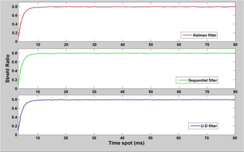
We use the sequential and U-D filters to compensate the wavefront distortion (Fig. 11). The results are quite similar with that of the Kalman filter, since they are basically constructed by the Kalman filter. The difference is that the sequential and U-D filters can avoid the matrix inversion which is complicated for the calculation for the embedded controller. This is important in the application but needs high speed processor.
It should be noticed that all the proposed filters do not aim at improving the SR or the coupling efficiency, or the similar metric in FSO system. Our filter is used to treat the unforeseen strong interference and to improve real-time ability of the FSO system. The other two proposed filters, sequential and U-D, can get the similar performance as the stand Kalman filter but they avoid the shortcoming of no convenient tool for matrix reversion in the realization of the embedded controller.
In this paper, various filters based on Kalman filters are introduced for discrete FSO-AO-loop system to compensate the dynamic wavefront distortion. From computer simulation, we find that the fading-memory filter is more responsive to current measurements than the standard Kalman filter, because it distributes more weight to the measurement at the current time step which avoids the divergence caused by the unforeseen pulse interference. Moreover, it is very simple to implement since we only add one parameter in the standard Kalman filter. Sequential filter and U-D filter are two acceptable algorithms suitable for an embedded system since they do not need matrix inversion, and the correcting results are comparable with the standard Kalman having tools for matrix inversion. These proposed algorithms are very useful especially for some real applications requiring counteracting the varied circumstances without human interference. Although they are at the cost of larger computational effort, rapidly improved hardware capability could effectively relieve this problem. Furthermore, all the modifications in the standard Kalman filter do not affect the operation of the AO system, which means that the stable continuous output signal can theoretically obtained by these filters.
In addition, all wavefront sensor based techniques, including our proposed methods, are not perfect to deal with strong scintillation, because the closed-loop bandwidth of these methods are in the level of dozens of Hertz, which cannot offer good performance when the Greenwood frequency is large. Moreover, strong intensity scintillations in the receiver aperture will make wavefront measurements difficult, mostly because of the occurrence of branch points in the optical field phase that results in a challenge for phase reconstruction techniques.
To deal with the strongly varied atmospheric turbulence, the wavefront sensor-less AO system is usually applied. It benefits from the recent development new efficient control algorithms, their implementation with parallel digital processing hardware based on VLSI microelectronics, and the emergence of high bandwidth, wavefront correctors based on microelectromechanical system (MEMSs). Due to the above explanations, in our paper, the generally constructed AO technology is used to deal with the weak and stationary turbulence [41].