Spectrum sensing plays an essential role in a cognitive radio network, which enables opportunistic access to an underutilized licensed spectrum. In conventional cooperative spectrum sensing (CSS), all cognitive users (CUs) in the network spend the same amount of time on spectrum sensing and waste time in remaining silent when other CUs report their sensing results to the fusion center. This problem is solved by the superposition cooperative spectrum sensing (SPCSS) scheme, where the sensing time of a CU is extended to the reporting time of the other CUs. Subsequently, SPCSS assigns the CUs different sensing times and thus affects both the sensing performance and the throughput of the system. In this paper, we propose an algorithm to determine the optimal sensing time of each CU for SPCSS that maximizes the achieved system throughput. The simulation results prove that the proposed scheme can significantly improve the throughput of the cognitive radio network compared with the conventional CSS.
In recent years, greater bandwidth and higher bit rates have been required to meet the increased usage demands caused by the explosion of wireless communication technology. According to the Federal Communications Commission spectrum policy task force report [1], the actual utilization of a licensed spectrum varies from 15% to 80%. Therefore, cognitive radio (CR) technology [2] has been proposed to solve the problem of the ineffective utilization of spectrum bands. The scarcity of spectrum bands can be relieved by allowing some cognitive users (CUs) to opportunistically access the spectrum assigned to the primary user (PU) whenever the channel is free. However, CUs must vacate their frequency when the presence of a PU is detected. Therefore, reliable detection of the PU signal is an essential requirement of CR networks.
To ascertain the presence of a PU, CUs can use one of the several common detection methods, such as the matched filter, feature, and energy detection methods [2,3]. Energy detection is an optimal detection method if the CUs have limited information about the PU signal (e.g., if only the local noise power is known) [3]. Improved spectrum usage detection can be obtained by allowing some CUs to perform cooperative spectrum sensing (CSS) [4-6].
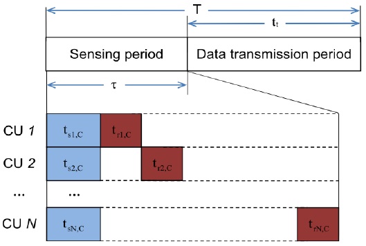
In conventional CSS, the time frame is divided into two main parts, namely the sensing and the data transmission parts. In the sensing part, all CUs take the same amount of time to perform spectrum sensing, and then, because of the limitations of the control channel, the CUs report their sensing results to the fusion center (FC) one by one, while the other CUs remain silent. On the other hand, the superposition cooperative spectrum sensing (SPCSS) proposed in [7], which allows CUs to extend their sensing times to the reporting slots of the others, can improve the sensing performance of CSS without requiring any more time for the sensing part. The trade-off between the sensing time and the throughput was studied in [8] for conventional CSS, in which the optimal sensing time for all CUs that maximize the throughput of the CR system was determined. Since the optimal sensing time obtained by [8] is the same for all CUs, it may not apply to SPCSS, in which each CU is assigned a different sensing time according to the reporting order of the CUs. Subsequently, the problem of determining the optimal sensing time for SPCSS is still open and needs more research on throughput maximization.
In this paper, we propose an algorithm to determine the optimal sensing time for SPCSS, with which the system can achieve the maximum throughput. In the proposed algorithm, we consider the reliability of the CUs (i.e., the signal-to-noise ratio (SNR) of the sensing channel) to decide the reporting order of the CUs. According to this order, the proposed algorithm determines the optimal sensing time for all the CUs in the network. Thus, we expect the proposed scheme to offer a higher throughput for CR networks than the conventional CSS scheme [8].
The rest of this paper is organized as follows: Section II describes the system model of the proposed scheme. Section III gives a detailed explanation of the proposed algorithm to find the optimal sensing time for maximizing the throughput of the CR system. Section IV introduces the simulation models and the simulation results of the proposed scheme. Finally, Section V concludes this paper.
In this study, we consider a network consisting of
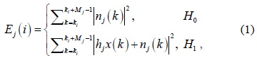
Each CU utilizes an energy detector for spectrum sensing. Then, at the

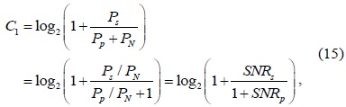
where
When
where
III. OPTIMAL SENSING TIME FOR SUPERPOSITION COOPERATIVE SPECTRUM SENSING
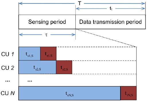
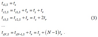
The sensing result (i.e. received signal power) that the CUs sense from the PU’s signal will be reported to the FC. In conventional CSS, when a CU sends the sensing results to the FC, the other CUs remain silent and wait until their reporting time. In this case, all the CUs have the same sensing time, as shown in Fig. 1, such that
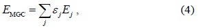
At the FC, a maximum gain combination (MGC) rule is used for combining all the sensing results from the CUs as follows:

where
Without any loss of generality, we assume that
>
A. Conventional Cooperative Spectrum Sensing
In the conventional CSS, all CUs have the same number of sensing samples (i.e., the same sensing time) such that

where
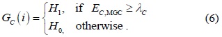
According to the value of

Here,
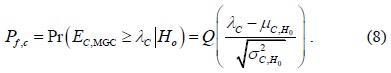
The sensing performance of the conventional CSS can be evaluated by the probability of detection and the probability of false alarm as follows, respectively:
and
>
B. Superposition Cooperative Spectrum Sensing
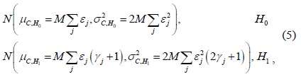
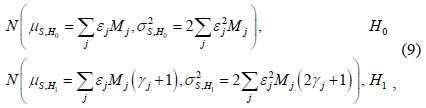
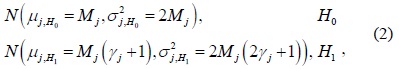
For the case of SPCSS, the CU that first reports its sensing information to the FC has the shortest sensing time, which is equal to the sensing time of conventional CSS. Other CUs will continue with spectrum sensing until their reporting rounds are reached. Therefore, different CUs will have a different number of sensing samples. Subsequently, the distribution of the accumulated signal power at the FC,

where
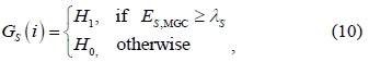
As in conventional CSS, in SPCSS, the global decision is made as follows:

where
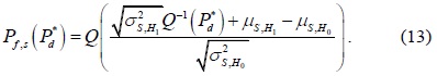
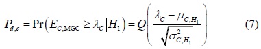
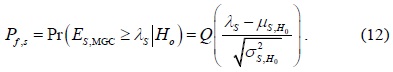
The sensing performance of the SPCSS can be evaluated by using the probability of detection and the probability of false alarm as follows, respectively:
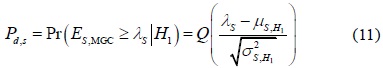
and
Depending on the required value of the probability of detection

Suppose that
Let us consider

and

where
Let us define

where
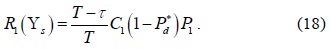
Further, Y
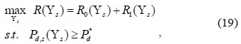
Next, the problem of determining the optimal sensing time can be formulated as follows:

where denotes the required probability of detection of the CR network.
Further, the reporting time
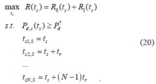
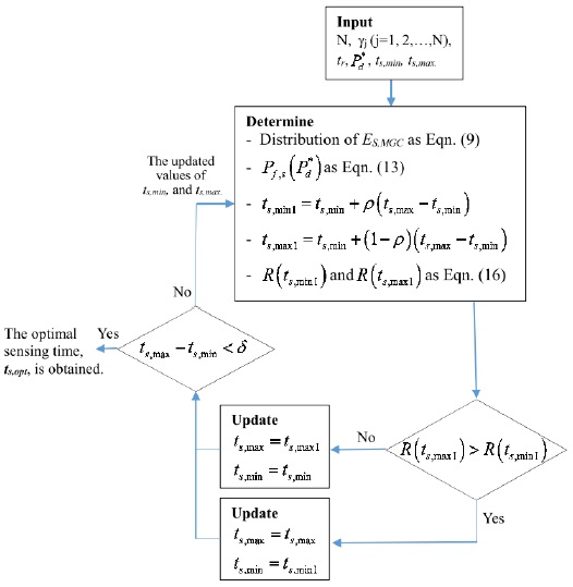
The problem in Eq. (20) can be solved to find the optimal sensing time
On the basis of this range, we apply the Golden search method to find
In this section, we will present the simulation results to demonstrate the performance of the proposed scheme. We consider a CR network containing 10 CUs and 1 PU with the absence probability of
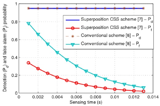
Fig. 4 shows the sensing performance at the FC of the CR network in terms of the probability of detection and the probability of false alarm
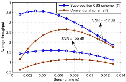
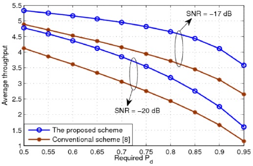
Fig. 5 presents the average throughput of the CR system for different values of the sensing time. It can be seen that SPCSS provides a considerable higher throughput than the conventional CSS. Further, at the same SNR in the sensing channel, the SPCSS needs a smaller sensing time to achieve the maximum average throughput than the conventional CSS. The average throughput of the CR system for different values of the required probability of detection is shown in Fig. 6. This figure proves that the proposed scheme can improve the throughput of the CR system. In other words, when the SNR of the sensing channel is –17 dB or –20 dB, the proposed scheme provides a throughput that is 30% or 40% higher than that of the conventional scheme, respectively.
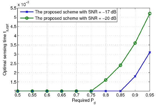
Fig. 7 shows the optimal sensing time
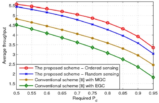
Fig. 8 shows the average throughput of the CR system for different values of the required probability of detection
In this paper, we proposed an algorithm to find the optimal sensing time of all the CUs for SPCSS. In the proposed algorithm, ordered sensing was considered for assigning a longer sensing time to the CUs with higher SNR values and a shorter sensing time to the CUs with lower SNR values. The simulation results showed that the proposed scheme could significantly improve the throughput of the CR system, in comparison with the conventional scheme [8]. Moreover, we observed that the proposed scheme with ordered sensing achieved a better performance than the proposed scheme with a random sensing order. However, further research is required to analytically prove this conclusion. This will be our future work on this research topic.